| Season | No PV | PV at 40% |
|---|---|---|
| Summer | 1.20 | 1.55 |
| Autumn | 0.54 | 1.59 |
| Winter | 0.77 | 1.15 |
| Spring | 0.57 | 1.84 |
Non-Technical Loss and Changes over Time
Chapter 2 found that no detector applied to a meter’s own readings detected under-recording reliably. The reason is structural rather than a weakness of the detectors: a register that records a constant share of the energy it should leaves the shape of each day unchanged, and a detector of the shape of a day has nothing to see. The energy that the meter does not record has not vanished, however. It still flows through the transformer that supplies the customer, and the transformer’s head measurement, compared with the sum of its customers’ meters, contains it. This chapter takes the anomaly from the level of the meter to the level of the transformer, where the energy balance makes it visible, and then turns to two further kinds of anomaly that a distribution network operator meets: behaviour that departs from the normal in its timing rather than its magnitude, and data or segments that no longer describe the network they were built on.
The chapter treats four problems. The first is non-technical loss: energy consumed and not billed, through a tampered register or a bypass of the meter. Its detection by the energy balance requires a model of the technical loss of the feeders, which grows with the square of the current, and the chapter shows that a model built on the head power alone fails once PV exports. The second is the irregular behaviour of an inverter, a meter clock or an EV charger, detected from the events of a day. The third is the cost of faulty readings to the decisions of Part 6, which a screening of the case base can limit for some faults and not for others. The fourth is whether the archetypes of Part 5 still describe the customers as they adopt PV and EVs, the question an operator must answer before it relies on a segmentation calibrated in an earlier period.
Each problem teaches a machine-learning idea on an LV problem, set against alternatives that rest on other assumptions.
Losses and Changes in the Literature
Non-technical loss is the part of the energy delivered to a network that is neither billed nor lost in its conductors. Messinis and Hatziargyriou reviewed its causes and the methods proposed for its detection, and Glauner and colleagues identified the scarcity of labelled cases as the principal obstacle to supervised detection [1], [2]. Supervised classifiers have been trained on consumption patterns with synthetic tampering [3], on features of smart-meter data from an operator’s inspections [4] and with deep convolutional networks on weekly consumption [5]. Their labels are mostly synthetic or come from inspections biased towards suspected customers, and their robustness to manipulated training data has itself become a subject of study [6]. Owners of distributed generation have an incentive of the opposite sign, to over-report their export, which Ismail and colleagues detected from the measured generation [7].
The energy balance needs no label. It compares the energy entering a part of the network with the energy its meters record, and attributes the difference beyond the technical loss to non-technical loss. Its difficulty lies in the technical loss itself, which a distribution network operator rarely measures and must estimate; Dashtaki and Haghifam estimated it in networks with limited data from the load and the network’s characteristics [8]. Faults of PV systems, the second problem of the chapter, have been reviewed by Mellit and colleagues, mostly from measurements inside the installation rather than from the customer’s meter [9].
The methods of the chapter rest on established statistics and machine learning. Detection from the residual of a model of normal behaviour is the analytical redundancy of fault diagnosis [10]; its fit can be made robust to contaminated data [11] or replaced by a flexible regressor such as gradient boosting [12], [13]. Attribution of a residual to one of many customers is a sparse regression [14], of which the score used here is one step of matching pursuit [15]. The power of the daily test follows from the theory of hypothesis tests [16], and the change of a customer’s behaviour over time is concept drift [17], [18], monitored by the cumulative sum of Page and the moving average of Roberts [19], [20]. Each problem is also one that operators meet on real networks: non-technical loss is a recognised share of distribution losses [1], inverters trip on over-voltage on Australian LV feeders with high PV penetration [21], and smart-meter records carry time-stamp errors, missing values and stuck readings [22].
Problem Formulation and Notation
A transformer \(j\) supplies the customers \(\mathcal{C}_j\). At each half-hour \(t\), its head measurement \(P^{\mathrm{head}}_t\), the active power at its secondary winding, equals the sum of the power its customers draw, less their PV export, plus the technical loss of its feeders. Customer \(i\)’s meter records \(P^{(i)}_t\), and a meter that under-records hides a share \(\eta\) of its customer’s demand \(D^{(i)}_t\). The balance
\[ P^{\mathrm{head}}_t = \sum_{i \in \mathcal{C}_j} P^{(i)}_t + P^{\mathrm{loss}}_t + u_t \tag{12.1}\]
defines the unexplained power \(u_t\), which is zero without tampering and equals \(\eta D^{(i)}_t\) when customer \(i\) under-records. A bypass, an appliance of power \(B\) connected ahead of the meter, adds \(B\) to the head power while it runs and leaves every meter unchanged, so that \(u_t = B\) during its use. The extra technical loss that the appliance’s current causes is of second order, about twice the loss share times \(B\), and is neglected. On a three-phase, four-wire secondary the balance holds for each phase \(\phi\) with the head power of the phase and the meters of the single-phase customers connected to it.
Technical loss is resistive and grows with the square of the current in each conductor. The head power is the net of the customers’ import and export, so the same head power can carry different currents: two models of the loss are compared,
\[ \hat P^{\mathrm{loss}}_t = a \left(P^{\mathrm{head}}_t\right)^2 + c , \tag{12.2}\]
from the head power alone, and
\[ \hat P^{\mathrm{loss}}_t = a \left(P^{\mathrm{head}}_t\right)^2 + b D_t^2 + g G_t^2 + c , \tag{12.3}\]
which adds the summed demand \(D_t\) and PV generation \(G_t\) of the customers, available from meters with separate import and export registers. Each model is fitted by least squares on days known to be normal. The daily unexplained energy \(U_d = \sum_{t \in d} u_t \, \Delta t\) of a test day is compared with the conformal threshold \(\hat q\) of the same statistic on calibration days, as in Equation 10.26, and the day is flagged when \(U_d > \hat q\).
| Symbol | Description |
|---|---|
| \(P^{\mathrm{head}}_t\), \(P^{(i)}_t\), \(P^{\mathrm{loss}}_t\) | Head power of a transformer or phase, the reading of customer \(i\), and the technical loss |
| \(D_t\), \(G_t\), \(D^{(i)}_t\) | Summed demand and PV generation of the customers, and the demand of customer \(i\) |
| \(u_t\), \(U_d\), \(\eta\), \(B\) | Unexplained power, unexplained energy of day \(d\), share of demand a meter hides, and power of a bypassed appliance |
| \(a\), \(b\), \(g\), \(c\) | Coefficients of the technical-loss models |
| \(\Gamma(i)\), \(\hat q\), \(\hat r\) | Conformal set of household \(i\), the conformal threshold (Part 5, Chapter 3) and the trust radius (Part 6) |
| \(d_{i,w}\), \(S_{i,w}\), \(h\) | Distance of household \(i\) to its archetype in week \(w\), its CUSUM statistic, and the decision limit |
Data and Protocol
The energy balance is computed on HPK11, the urban network of AusNet with 44 LV transformers and 5,274 customers on which Parts 5 and 6 are built, from a registered power flow (balance). Every customer follows the measured demand of its assigned AusNet household, and the PV systems of 40% of the residential customers, drawn at random, follow AS/NZS 4777.2 with volt-VAr and volt-watt response, as in Part 5. The flow is solved for the four seasonal weeks of the other simulations, without PV and with PV, and records for every phase of every transformer and every half-hour the head power, the demand and PV output of the customers on the phase, and the technical loss of its feeders. Each residential customer is connected to the phase given by the node of its bus, and the one three-phase customer counts a third on each phase. Every step of the solution converged, and the loss of the feeders was 0.54 to 1.20% of the customers’ demand without PV and 1.15 to 1.84% with PV (Table 12.2). Transformers with fewer than five customers are excluded, since their balance is dominated by a single meter.
Tampering changes what a meter records or what the head carries, not the physics of the network, so it is injected into the balance after the solution: one customer of a transformer hides 30, 50 or 70% of its demand for a whole week, or runs an appliance of 1 or 2 kW connected ahead of its meter from 17:00 to 22:00 every day of the week, a load of the size of an electric heater or a hot-water system. The evaluation holds out one week at a time. The loss model and the threshold are fitted on the other three weeks, so that a held-out week is a different season from every calibration day, as it would be for an operator who calibrates on past data. With no customer tampering, the share of days flagged is the false-alarm rate, whose target is 10%. Three customers per transformer tamper in turn. Comparisons between methods on the same transformers, weeks and customers are tested with the Wilcoxon signed-rank test of the paired results.
The Energy Balance of a Transformer
Technical Loss and the Residual
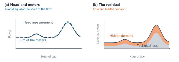
The meters of a transformer do not sum to its head measurement even when none is tampered with, because the feeders between them dissipate energy in their resistance (Figure 12.1). The difference is small against the flow, about one percent in Table 12.2, but it is of the same order as the energy that one tampering customer hides, and it varies from half-hour to half-hour with the square of the current. A test of the raw difference would therefore flag the days of high load, on which the loss is high, rather than the days of tampering. The loss must be modelled and subtracted first, and what remains, the residual \(u_t\) of Equation 12.1, is the quantity that the balance tests.
The loss was larger with PV in every season, 1.15 to 1.84% of demand against 0.54 to 1.20%, although PV reduces the energy the transformer delivers. The reason is the cancellation of import and export in the head power. At midday, an exporting customer and an importing customer on the same feeder drive currents in opposite directions through the shared conductors near the transformer, and their sum at the head can be small while each branch carries its full current. The loss follows the branch currents, not their sum, so the head power ceases to be a sufficient description of the loss once customers export. Figure 12.2 shows this on the most populous transformer of HPK11: without PV the loss is a single curve in the head power, while with PV the half-hours of export lie above that curve, carrying a larger loss at the same head power.
NoteRemark for the machine-learning reader
The technical loss plays the role of a known nuisance term. It is not anomalous, it is present every day, and its size is comparable with the effect to be detected. A detector applied to the raw residual would learn the loss and flag its peaks. Subtracting a physical model of the nuisance before testing is the regression analogue of removing a seasonal component before detecting anomalies in a time series: the test is then made on what the model cannot explain, and its power depends on how much of the nuisance the model removes.
The test is a residual-based detector [10]. With \(\hat f\) the loss model fitted on normal steps, the daily statistic
\[ U_d = \sum_{t \in d} \left(P^{\mathrm{head}}_t - \sum_i P^{(i)}_t - \hat f(x_t)\right) \Delta t \tag{12.4}\]
is compared with the conformal threshold of the same statistic on calibration days. The test holds its false-alarm rate under three assumptions: the model is correctly specified, so that \(U_d\) has no systematic part; the residuals of calibration and test days are exchangeable; and the calibration days are free of tampering. The sections that follow show each assumption failing on HPK11.
NoteRemark for the power-system reader
Technical loss is the \(I^2R\) heating of every conductor between the transformer and the meters, so it depends on the current in each branch, including the neutral conductor that carries the unbalance between phases. A loss model in the head power alone assumes that the head current describes the branch currents, which holds when every customer imports and fails when some export.
A Worked Example
The size of the signal follows from the balance. Consider the HPK11 transformer nearest 120 customers, which has 123, without PV. In the four weeks it delivered on average 1,972 kWh per day, of which 16.9 kWh was technical loss. A customer of 4 MWh a year who hides half its demand removes 5.5 kWh per day from the meters, 0.28% of the energy through the transformer, and a third of the daily loss. A test of the raw difference would see this as a 33% rise in the loss, within the day-to-day variation of the loss itself between seasons. After the import-and-export loss model of Equation 12.3 is subtracted, however, the daily residual of the normal days had a standard deviation of 0.50 kWh and a 90% conformal threshold of 0.80 kWh, so the hidden 5.5 kWh is about eleven standard deviations of the residual. The worked example shows the two quantities that determine detection: the energy hidden, which is a property of the customer, and the spread of the residual after the loss model, which is a property of the transformer and of the model. A customer hiding a third as much on a transformer three times as large would be at the threshold.
Detection of Under-Recording and Bypass
The Loss Model Decides the False-Alarm Rate
Table 12.3 reports the share of days flagged across the 44 transformers. With the import-and-export loss model, the false-alarm rate was 10.3% without PV and 9.3% with PV, close to the target of 10% although every held-out week was a season absent from calibration. One customer hiding 30% of its demand was flagged on 78.6% of days without PV and 79.0% with PV, and hiding 70% on 91.6% and 92.2%. The head-only model of Equation 12.2 behaved differently with and without PV. Without PV it flagged more tampered days, 90.3% at 30%, but its false-alarm rate was 16.4%, so its higher detection was bought with a threshold that its own calibration no longer held. With PV its false-alarm rate rose to 22.0% and its detection at 30% fell to 34.9%. Both differences between the two models were significant on the paired transformer-weeks (Wilcoxon \(p < 10^{-6}\) for the false alarms and \(p < 10^{-24}\) for detection at 30%, with and without PV).
The rates translate into the workload of an operator. A false-alarm rate of 10% on 44 transformers flags about four transformers on a normal day, so a daily flag is a reason to watch a transformer rather than to inspect it. A customer hiding 30% of its demand is flagged on about four days in five. If days were independent, a normal transformer would be flagged on four or more of seven days with probability 0.3%, and a weekly count would be an almost certain decision. It was not: a normal transformer was flagged on four or more days in 8.7% of weeks without PV and 3.5% with PV, while one hiding 30% of demand was found in 76.6% and 80.8% of weeks. The days of a held-out season share its departure from the calibration seasons, so false alarms come in runs, and a weekly decision adds little to a daily one. The head-only model with PV makes either decision unreliable, since it flags one normal day in five and misses two tampered days in three.
The two failures of the head-only model have one cause. A misspecified loss model leaves part of the loss in the residual, and that part varies between seasons, because the share of export varies. The residual of the calibration weeks is then wider than it would be under the correct model, which lowers the detection, and the residual of a held-out season is shifted from that of the calibration seasons, which raises the false alarms. The import-and-export model needs only what a meter with separate registers already records, so the remedy for an operator with such meters costs no measurement. The implication extends beyond loss: a conformal threshold guarantees its false-alarm rate only for residuals exchangeable with the calibration residuals, and a model that omits a seasonal driver breaks that exchangeability without any change in the network.
Figure 12.3 shows the test on the worked example. The unexplained power of the tampered winter week follows the hidden demand, with its evening peaks, above the residual of the same week without tampering. Each tampered day lay above every one of the 21 calibration days, which spread around zero within the threshold.
Bypass of the Meter
A bypass leaves the meter readings intact and adds its load to the head. With the import-and-export model, an appliance of 1 kW run for five evening hours was flagged on 86.7% of days without PV and 86.3% with PV, and one of 2 kW on 90.1% and 92.4% (Table 12.4). The energy of a 1 kW bypass, 5 kWh per day, is close to that hidden by the customer of the worked example, and it was detected more often than an under-recording of 30% because it does not shrink on the days of low demand. The head-only model again failed with PV, flagging 41.4% and 62.6% of days. In terms of energy, a 1 kW bypass for five evening hours is about 1.8 MWh a year, the consumption of a small household taken without payment, and the balance finds it within a week on almost every transformer of HPK11. The balance does not distinguish the two kinds of tampering, since both appear as unexplained energy; the distinction is made at the site visit, and the timing of the residual, concentrated in the evening for an appliance and proportional to the customer’s demand for a register, indicates which to expect.
Loss Models Learned from Data
A physical loss model needs the import and export of the customers; a data-driven model needs only the records. Gradient-boosted trees fitted on the head power, the summed import and generation and the hour of the day [12] detected one customer hiding 30% of its demand on 95.0% of days without PV and 96.3% with PV, more than the physical model’s 77.9% and 77.1%, but flagged 27.9% and 33.8% of normal days against the target of 10% (Table 12.5). The trees fit the calibration weeks closely, so the residuals on which the threshold is calibrated are smaller than the residuals of a new week, and the threshold is too low. A split-conformal threshold requires residuals the model has not been fitted on; calibrating a flexible model on its own training residuals breaks the guarantee, while a linear model with four coefficients barely overfits and keeps it. The robust Huber fit of the physical model [11] behaved as least squares did, with false alarms of 11.1% and 9.6%.
The third assumption, clean calibration days, is the one an operator can least verify. When the tampering customer also hid 30% of its demand in one of the three calibration weeks, detection with least squares fell from 77.9% to 27.4% without PV and from 77.1% to 31.9% with PV: the loss model and the threshold absorbed part of the hidden demand as if it were technical loss. The Huber fit recovered almost nothing (28.8% and 33.5%), because robust regression down-weights scattered outlying steps, and a customer who tampers throughout a week is not an outlier but a shift of a whole block of steps. For an operator, the consequence is that a balance calibrated on a period that already contained the tampering will not find it; the calibration period is chosen after an inspection, or a long one is used so that a tampering customer is a small part of it.
Pitfall: calibrating a flexible model on its own training residuals
A flexible regressor reduces the residual on the steps it is fitted on, and a threshold calibrated on those residuals is too low for new steps. The conformal guarantee holds only for residuals of steps held out from the fit; with a flexible loss model, part of the normal days must be set aside for calibration.
Detection and the Size of the Transformer
The worked example implies that detection falls with the number of customers, since a larger transformer has a larger residual spread for the same hidden energy. If the tampered day’s residual is a normal day’s residual plus the hidden energy \(h_d\), the probability that the day is flagged is
\[ \Pr(U_d > \hat q) = \Pr(U^{0} > \hat q - h_d), \tag{12.5}\]
where \(U^{0}\) is a normal day’s residual, so the power of the test is read from the calibration residuals alone [16]. Figure 12.4 compares this prediction with the observed detection. Every transformer lay below the line of agreement, by 0.17 on average: the held-out season’s residual was wider than the calibration seasons predicted, the exchangeability assumption of Equation 12.4 failing across seasons. The prediction ranks the transformers correctly and overstates their detection, so an operator uses it to choose where the balance is worth installing and not to promise a detection rate.
Figure 12.5 confirms it. At 30% hidden with the import-and-export model, the mean share of days flagged was 82.1% on transformers of fewer than 60 customers, 80.5% on those of 60 to 120 and 76.6% on larger ones without PV, and 98.4%, 86.9% and 69.2% with PV. The decline was steeper with PV because export adds a component of the loss that varies with the weather, which the model captures only in part. For an operator, the relation states where the balance is most informative: on small and medium transformers, and on large transformers only for larger hidden shares or with a longer test window than one day. With PV the large transformers lost most, from 98.4% to 69.2%, which means that the transformers of new estates, large and with high PV penetration, are where a daily balance misses most tampering, and where a weekly test, which sums seven days of hidden energy against a residual whose spread grows only with the square root of seven, recovers it.
The comparison with Chapter 2 is direct. The self-baseline detectors of that chapter, applied to each meter’s own readings, did not detect an under-recording of half of every reading reliably with any representation of a day, because the under-recorded day has the shape of a normal day at a lower level. The balance detected a third of that fault on four days in five. The two approaches see different evidence: the meter’s history cannot distinguish a lower reading from a lower demand, while the balance compares the reading with the energy that was delivered.
Pitfall: a loss model fitted on the head power alone
A model of technical loss in the head power is adequate for a network without export, and an operator who calibrated it before PV was installed will see it perform well. Once customers export, import and export cancel in the head power but not in the feeders, and the model leaves a seasonal share of the loss in the residual. The threshold then flags a growing share of normal days, while tampering in the season of most export goes undetected. A loss model is refitted with separate import and export terms whenever the penetration of PV changes.
Narrowing the Search to a Customer
A flagged transformer does not identify the customer. The residual of a tampering customer is a hidden share of its demand, \(r_t = \beta_i d_{i,t} + \varepsilon_t\), so attribution is a sparse regression of the residual on the demand of every customer with a single non-zero share [14]. The score
\[ s_i = \max\left(0, \frac{\langle d_i, r \rangle}{\langle d_i, d_i \rangle}\right) \operatorname{corr}(d_i, r) \tag{12.6}\]
fits each customer alone, one step of matching pursuit [15]. A site visit to each of a hundred customers is not a practical response, so the operator needs an order of visits. The residual of a tampering customer follows its demand in time, scaled by the hidden share, and the score of umeme.losses.locate regresses the residual of the flagged week on each customer’s demand, keeps the positive share and weights it by the correlation, so that the customer whose demand best explains the residual is visited first. On HPK11 without PV, with one customer hiding 30% of its demand, the tampering customer ranked first in 75.6% of 172 transformer-weeks, and within the first five in 90.7%, on transformers with a median of 125 customers (Figure 12.6). Without the score, a crew visiting the customers of such a transformer in random order would need 63 visits on average to find the tampering customer; with it, three times in four the first visit suffices, and nine times in ten the first five. The score therefore converts a flag of the balance into a short list of customers, which is what makes the balance usable for revenue protection rather than only for reporting. The score works because the demand of each household has its own timing: two households rarely share the hours of their peaks over a whole week, and the residual inherits the timing of the one that hides demand.
Fitting all customers jointly, by non-negative least squares or by the non-negative lasso with its penalty chosen by BIC, found more tampering customers (Figure 12.7): on the first visit 80.8% with non-negative least squares and 80.2% with the lasso against 75.6% with matching pursuit, and within five visits 96.5% with the lasso against 90.7% with either of the others. The lasso’s preference for few non-zero shares matches the structure of the problem, one tampering customer among many, which is why it gained most. A joint fit separates customers whose demand overlaps, which the score of Equation 12.6 cannot. Every method failed where another customer’s demand had the same timing as the tampering customer’s, and some customers of the simulation share a measured household: HPK11 assigns 342 AusNet households to 5,274 customers, so two customers of a transformer can have identical demand, and no attribution from the readings can tell them apart; this was the case in 41 of the 172 transformer-weeks, which bounds every method’s recall in this simulation. On a real network two households rarely draw identical demand, but households of similar habits are common, and the correlation of a customer’s demand with its neighbours’ bounds how well any attribution can work.
Where the head is measured per phase, the search can be restricted first to the customers of the phase whose residual holds the largest unexplained energy. The phase was the tampering customer’s in 89.5% of weeks, and visiting its customers first in the same order found 77.3% of tampering customers on the first visit, slightly more than the whole transformer, but 84.3% within five visits, fewer, and the median rank did not differ (Wilcoxon \(p = 0.90\)). In one week in ten the largest unexplained energy appeared on another phase, and a customer whom the whole-transformer score would have found at once was then reached only after every customer of the wrong phase. The residuals of the phases are not independent: the loss in the shared neutral conductor and the unbalance between phases couple them, and a per-phase loss model attributes part of one phase’s loss to another.
Pitfall: restricting the search to one phase
A per-phase measurement appears to reduce the search to a third of the customers. The restriction is only as reliable as the identification of the phase, and an error sends the visits to a group that does not contain the tampering customer. The score of the whole transformer already exploits the timing of each customer’s demand, which is the stronger evidence. The phase is used to order customers of equal score, not to exclude the other phases.
Irregular Export of Inverters and Irregular Charging
Faults That Change Timing, Not Energy
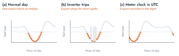
Chapter 2 detected faults that change what a meter records. A second class changes when the recorded energy occurs. An inverter that trips repeatedly on the over-voltage or anti-islanding protection of AS/NZS 4777.2 stops exporting for short spells and resumes, and during each spell the household imports its demand. A meter whose clock records UTC as local time labels every reading ten hours early in Victoria, so that the midday export of a household appears in the night (Figure 12.8). EV charging shows the same two forms: a session broken into fragments, and a session moved to another part of the day by a misconfigured timer. None of these faults changes the day’s energy much, and a detector of magnitude, which describes a day by its total, its extremes and its spread, has little to see.
Each customer’s days are scored by an Isolation Forest [23], which isolates a day by random axis-parallel splits of its features and scores it by how few splits isolate it, assuming that anomalies are few and different. The hour of an event enters through its circular mean,
\[ \bar\theta = \operatorname{atan2}\left(\sum_t \sin\theta_t, \sum_t \cos\theta_t\right), \quad \theta_t = 2\pi h_t / 24, \tag{12.7}\]
which places an episode from 22:00 to 03:00 at midnight, where the arithmetic mean of its hours places it near noon [24]. The faults were injected into five later days of each of 120 AusNet households with PV of 3 to 8 kWp, and of the 200 charging series of the network simulations, which were synthesised from statistics of Norwegian charging sessions; measured sessions of individual drivers are used in Part 8. Each customer’s Isolation Forest was fitted on its own earlier days, 180 for export and 240 for charging, and the day was described in one of three ways: by its magnitude, by the events of its export or charging (occurrence, number of episodes, severity, and hour of start and end) with the clock hour, or by the same events with the hour on the 24-hour circle, as in Chapter 1.
Events and the Circular Hour
Table 12.6 reports the median AUC across customers. The magnitude representation detected none of the export faults, with median AUCs of 0.375 for trips and 0.507 for the clock error, at or below chance, and only part of the charging faults, 0.690 and 0.742. The events detected both kinds. Trips were detected with a median AUC of 0.702 with the clock hour and 0.728 with the circular hour, and fragmented charging with 0.963 and 0.955. A trip shortens the export and adds episodes, which the event counts register, but a single short trip on a cloudy day resembles the household’s own cloudy days, and the AUC is accordingly lower than for charging, whose sessions are otherwise regular. An AUC of 0.73 means that a tripping day outranks a normal day of the same household in about three comparisons of four: enough to rank the households whose inverters most likely trip, for a check of their voltage at the point of connection, not enough to act on a single day. Repeated trips on a household are themselves evidence of a network problem, since the over-voltage protection of AS/NZS 4777.2 trips when the voltage at the inverter exceeds its limit, so the households ranked highest point to the feeders where the voltage rise of Part 5 constrains export.
The faults that move the behaviour in time separated the two encodings of the hour (Figure 12.9). The clock error was detected with a median AUC of 0.884 with the clock hour and 0.947 with the circular hour, and the moved charging with 0.790 and 0.881; both differences were significant across customers (Wilcoxon \(p < 10^{-16}\)). An export recorded in the night, and a session moved past midnight, straddle the boundary of the clock, where the mean of the clock hour of an episode from 22:00 to 03:00 is near noon and coincides with that of a normal day. On the circle the same episode lies at night, far from the midday of normal export. A clock error is not a theft, but it corrupts every time-of-use bill and every half-hourly profile drawn from the meter, so a detector with a median AUC of 0.95 makes it practical to screen a whole meter population for clock faults before the readings are used in the segmentations of Part 5 or the studies of Part 6. The representation of time is therefore part of the detector: a feature that is periodic must be encoded as periodic, or the faults that move behaviour across midnight are hidden by the encoding.
Figure 12.10 shows two flagged days of one household. On the day of trips the export stops twice in the early afternoon and the household imports; on the day of the clock error the export lies between midnight and 08:00 and the evening import lies at midday. In both, the energy of the day is within the band of the household’s normal days, and the departure is in the timing of the export.
Whether the gain came from the representation or from the detector is settled by a second detector on the same representation (Table 12.7). The local outlier factor [25] on standardised features raised the median AUC of inverter trips from 0.728 to 0.846 and of the meter clock error from 0.947 to 1.000, and matched the Isolation Forest on EV charging; one Isolation Forest pooled over every customer was close to one per customer. The representation decided whether a fault could be seen at all, from chance with magnitude to 0.95 with events, and the detector decided how much of it was seen: an inverter trip changes a few features of a day by a little, which a density-based detector resolves better than random splits.
Figure 12.11 shows the detector on one household’s held-out days, with the threshold calibrated on 60 earlier days the detector did not see. All five injected days were flagged, but normal days were flagged more often as the held-out days moved from the calibration season towards winter. The detector is calibrated on a season, and an operator recalibrates it as the seasons change, as Chapter 2 found for the meters.
NoteRemark for the power-system reader
An inverter disconnects when the voltage at its terminals exceeds the limit of its protection, and reconnects after a delay, so repeated trips on a sunny day point to a feeder where the voltage rise of Part 5 already constrains export. A meter clock error is a configuration fault of the metering system rather than of the customer, and it shifts every interval reading of the meter, which corrupts any analysis that relies on the time of day.
Faulty Readings in the Decisions of Part 6
A fault that is not detected enters the decisions built on the readings. Part 6, Chapter 2 estimated the contribution of a customer to the evening peak of its transformer from its ten nearest cases by size of demand. Here a share of the kept households’ readings was corrupted by one of three faults (a register stuck at one value, dropouts to zero, or under-recording of a third of every reading), the estimate was recomputed for held-out customers, and the error was compared with the estimate from clean readings over 30 random splits (Table 12.8). The screening applied the repeat ratio and the runs of zeros of Chapter 2, which passed 90.1% of the clean AusNet meters.
Stuck registers and dropouts barely changed the decision: with 30% of the case base faulty, the error of the peak contribution was 1.615 kW against 1.613 kW from clean readings, and Kendall’s \(\tau\) 0.151 against 0.154, with no paired difference across splits (\(p > 0.3\)). A stuck run or a dropout affects a few days, and the size features of a household, averaged over a year, absorb them. Under-recording at 30% raised the error from 1.605 to 1.733 kW and lowered \(\tau\) from 0.151 to 0.096 (\(p < 10^{-8}\)), because it shifts every reading of a household and moves it to the neighbourhood of smaller households. An increase of 0.13 kW per customer is 8% of the error, and on a transformer of 100 customers it is 13 kW of peak contribution misestimated, of the order of the headroom on which a connection assessment of Part 6 decides. Each size feature is a mean over the days of the year, \(\bar x_i = \frac{1}{n}\sum_d x_{i,d}\), so a fault on \(m\) of \(n\) days moves it by about \(m/n\) of the fault’s size, while an under-recording of a share \(\eta\) moves it by \(\eta \bar x_i\) whatever \(n\) is. Random faults average out of the features; a systematic one does not. Figure 12.12 shows the consequence for the estimates: the whole distribution of errors moved upward, its median from 0.60 to 0.73 kW, because the faulty households looked smaller and the queries were matched to cases whose contribution was larger. Screening did not recover the loss: the screened case base had an error of 1.731 kW (\(p = 0.90\) against the corrupted one), since an under-recording meter passes every rule of validation. The value of a screening is therefore set by the decision it protects. The faults that validation rules find cost the retrieval of Part 6 little, and the fault that costs most is the one that only the energy balance of the transformer reveals. A rank correlation of 0.15 between estimated and simulated contributions, from size features alone, is weak in either case, and the result concerns the change caused by faults rather than the quality of the estimate.
A representation invariant to the fault removes it at a price. Described by the shape of their mean day, which a constant under-recording does not change, the households gave the same error from a clean and from an under-recording case base, 1.747 kW in both, but a larger error than the size features gave from clean readings, 1.613 kW. Invariance to a fault discards the information the fault corrupts, and here that information, the size of the demand, is what the estimate needs; the operator’s remedy is to find the under-recording meters, by the balance of this chapter, rather than to remove from the retrieval the information they corrupt.
Whether the Segments Still Describe the Customers
Membership and the Trust Radius under Adoption
The archetypes of Part 5 were fitted to readings of one period, and a decision built on them, a tariff, a representative profile or a calibrated threshold, assumes that they still describe the customers. As customers install PV or charge an EV, their demand moves away from every archetype. The conformal membership set of Part 5, Chapter 3 (Figure 5.14) measures this directly: a household is described when at least one archetype’s centroid lies within the calibrated distance \(\hat q\), which holds for about \(1 - \alpha\) of households before adoption. The sets are computed here in the space of seasonal profiles from which the archetypes were built, since the t-SNE embedding of Part 5 cannot place new readings.
Before adoption, 91.5% of the 342 AusNet households were described, at the nominal 90%. As a growing share adopted a mix of Level 1 and Level 2 EV charging, PV of 3 to 8 kWp, or both, the share described fell to 83.3% at 20% adoption, 71.6% at 40% and 56.1% at 80% (Figure 12.13). The trust radius of Part 6, the conformal distance to the nearest household of the reference rather than to an archetype, fell in the same way, from 97.4% of households within it to 87.7%, 75.4% and 59.1%. Both measures state the same limitation: a segmentation, or a case base, calibrated before adoption describes a shrinking share of the customers after it. At 40% adoption, more than a quarter of households had no archetype within the calibrated distance. For those households a tariff or a representative profile assigned by archetype rests on no evidence, and a network study that represents them by their archetype’s profile misses the midday export and the evening charging that their readings now contain. The share described is thus a direct indicator of when the segmentation must be refitted: once it falls well below the nominal \(1 - \alpha\), here already at 20% adoption, the archetypes no longer support decisions.
Pitfall: identical adoption that raises apparent trust
When every adopter installed the same Level 2 charger, the share described rose, from 91.5% to 95.6% at 80% adoption, and the share within the trust radius from 97.4% to 98.2%. The households did not resemble the archetypes more: identical adoption added the same evening block to every adopter’s profile, which made the adopters resemble one another and moved their profiles towards the dense region of the calibration households. A study that models adoption as a single representative technology will conclude that the segmentation remains valid, when a mix of technologies, as observed on real networks, erodes it.
Detecting the Week a Household Changes
Adoption is covariate drift in the sense of machine learning: the distribution of the customers’ features moves while the archetypes, the concept, stay as they were [17], [18]. The conformal guarantee of the membership sets assumes that new households are exchangeable with the calibration households, and drift removes it. The membership set compares a whole period with the reference. An operator also needs to know when, within a year, a household stops resembling its archetype, so that a model can be refitted before its decisions degrade. Let \(d_{i,w}\) be the Euclidean distance between household \(i\)’s peak-normalised mean daily profile in week \(w\) and its archetype’s mean profile of the same week, which removes the seasonal pattern common to the archetype. Standardised by the household’s mean \(\mu_i\) and standard deviation \(\sigma_i\) over a baseline of 16 weeks, the one-sided CUSUM
\[ S_{i,w} = \max\left(0,\; S_{i,w-1} + \frac{d_{i,w} - \mu_i}{\sigma_i} - k\right) \tag{12.8}\]
with allowance \(k = 0.5\) accumulates sustained departures and forgets isolated ones [19], and the household is alarmed in the first week in which \(S_{i,w} > h\). Real households drift from their archetype through the year for reasons other than adoption, and a limit set from the nominal run length of the CUSUM alarmed a quarter or more of households that did not adopt. The limit \(h\) was therefore calibrated as the split-conformal quantile of the largest statistic reached over the monitored weeks by 30% of households held out without adoption, the construction of Equation 10.26 with the maximum of the path as the score.
If the households without adoption are exchangeable with the calibration households, the calibrated limit \(h\) satisfies \(\Pr(\max_w S_{i,w} > h) \le \alpha\) for a new household without adoption, which bounds its probability of an alarm within the horizon. The nominal limit of the CUSUM, \(h = 5\) standard deviations, alarmed 47.8% of the households that did not adopt within the half-year, nearly five times the target, because the weekly distances of a household are correlated and drift with the seasons, against the independence the nominal run length assumes. A quarter of the 240 monitored households adopted a technology on 1 July. Of the households that did not adopt, 15.0% were alarmed within the half-year, near the 10% target given 102 calibration households, and 1.7% of adopters were alarmed before their adoption. PV was detected in 93.8% of adopters with a median delay of two weeks, and PV with Level 2 charging in all, also within two weeks (Figure 12.14). Level 2 charging alone was detected in 66.7% of adopters after a median of 15 weeks, and Level 1 charging in 14.3%. PV changes the shape of every day, since the midday import becomes export, while charging adds a block on the evenings of a few days a week, which the weekly mean dilutes; Level 1 charging at 2.4 kW is a small departure even on those days. For an operator the result means that a segmentation can be kept current for PV by a weekly check of each household, whose alarms identify the new PV owners within a month, which can precede the update of the connection record in the network model; for EV charging the same check identifies two Level 2 owners in three only after a season, which is too late for the evening peaks of the first winter. Figure 12.15 shows a PV adopter whose statistic crossed the limit within two weeks of adoption, against a household of the same archetype that did not adopt.
Figure 12.16 sets the alarms against the true adoption for a sample of households of each technology. An exponentially weighted moving average of the same distance [20], calibrated in the same way, alarmed the same 15.0% of households without adoption and found slightly fewer adopters, 87.5% of PV adopters against 93.8% and 60.0% of Level 2 EV adopters against 66.7%: the moving average forgets the early weeks of a slow change that the CUSUM accumulates.
NoteRemark for the machine-learning reader
The nominal limits of a CUSUM or an EWMA chart assume independent observations of known spread, the setting of industrial process control. Calibrating the limit on held-out units without change, as here, is a conformal construction on the largest statistic of a path, and it transfers the guarantee to correlated, drifting series at the cost of a held-out sample of units.
The monitor answers the question of when to refit a segmentation for PV, which it detects within weeks, but only partly for EV charging. A shape-based distance is the wrong statistic for a technology that adds energy on some evenings: the events of charging of the previous section, or the energy of the evening hours, are the statistics that charging changes, and the same CUSUM applied to them is the corresponding monitor.
Further Applications
The methods of this chapter apply to other problems of an LV operator. The energy balance with a physical loss model is the basis of loss allocation between the technical and the commercial, which regulators of several countries require operators to report; the import-and-export model of Equation 12.3 gives the technical share per transformer with PV, from the meters the operator already holds, and the detection threshold of Equation 10.26 gives the share that cannot be attributed to the loss with a stated confidence. The same balance validates the network model itself. A persistent residual on a transformer without a tampering customer indicates a customer assigned to the wrong transformer or phase in the operator’s records, or a conductor of another impedance than recorded; Part 5, Chapter 6 identified phases from voltage correlation, and the balance per phase tests the identification with energy. A residual that appears on all the transformers of a feeder at once indicates a fault of the head measurement rather than of a customer.
The events of a day, encoded with the circular hour, detect other faults of timing that a utility meets. A meter whose clock moved by one hour at the change to daylight saving time shifts its readings by an hour on one date, and the detector of this chapter applies with a shift of two half-hours. A household battery that charges from the grid at night after a change of its schedule, or an export limit that clips the midday export of a PV system after a firmware update, change the events of export and not its energy. For EV charging the same representation detects a charger that ignores the off-peak window of a tariff, which is a question of compliance with a time-of-use agreement, and a public charger whose sessions fragment because of a communication fault.
The calibrated CUSUM of Equation 12.8 is a general monitor of drift for the models of Parts 5 and 6. Applied to the distance of each transformer’s daily violation events to their violation pattern, it detects when a transformer leaves its violation pattern of Part 5, Chapter 4; applied to the error of the case base of Part 6 on new studies, it detects when the case base no longer represents the requests it receives. In each case the decision limit is calibrated on units known not to have changed, and the alarm triggers a refit or a new study rather than an inspection.
Conclusion
This chapter moved the detection of anomalies from the meter to the transformer and from the day to the period. Non-technical loss that no meter shows was revealed by the energy balance between the head measurement and the meters, once the technical loss of the feeders was modelled. A model of the loss in the head power alone failed with PV, because import and export cancel in the head power but not in the feeders: its false-alarm rate rose from the target of 10% to 22.0% and its detection of a 30% under-recording fell to 34.9%. A model with the import and export registers that meters already record held the false-alarm rate at 9.3 to 10.3% and detected the same under-recording on 79% of days and a bypassed appliance of 1 kW on 87%, with detection falling as the transformer grows, as the worked example predicts. The score of each customer’s demand against the residual found the tampering customer on the first visit in three cases of four; a restriction to the flagged phase did not improve on it.
Faults of an inverter or a meter clock, which change the timing of export rather than its energy, were invisible to magnitude and detected by the events of a day, and those that move behaviour across midnight required the hour to be encoded on the circle. Faulty readings that validation rules detect cost the retrieval of Part 6 little, while under-recording, which passes every rule, cost most and was not removed by screening. The archetypes of Part 5 described a falling share of households as a mix of technologies was adopted, from 91.5% to 56.1% at 80% adoption, while identical adoption appeared to raise the share described. A CUSUM calibrated on households without adoption detected PV adoption within two weeks and EV charging only partly.
The limitations follow from the data. Tampering was injected into a simulated balance, so the residual contained no metering error of the head measurement or of the meters’ classes of accuracy, which would widen the residual and lower detection; the bypass neglected the extra loss its current causes; and the EV series were synthesised rather than measured per driver. Chapter 4 turns from the customer to the network itself: anomalies that appear only in the coincidence of many customers, and violation events that depart from their violation pattern.
Exercises
- Show from Equation 12.3 that two customers on the same feeder, one importing \(P\) and one exporting \(P\), give a head power of zero and a loss that the head-only model of Equation 12.2 predicts as \(c\). Compute the loss they cause on a feeder of resistance 0.05 Ω at 230 V for \(P = 3\) kW.
- Repeat the worked example in the
examplecell for the largest transformer of HPK11, and state the share of demand that a customer of 4 MWh a year must hide to reach the conformal threshold. - In the
detectioncell, calibrate the threshold on the other three weeks pooled with the first three days of the held-out week. How do the false-alarm rates of the head-only model with PV change, and which assumption of Equation 10.26 does the change restore? - Change the bypass in
umeme.losses.BYPASSto a load running from 01:00 to 06:00, as an EV charged ahead of the meter. Is it detected more or less often than the evening appliance, and why does the season of the week matter? - In the
locatecell, visit the customers of the flagged phase first only when its unexplained energy exceeds that of the other phases by a factor of two, and the whole transformer otherwise. Does the rule recover the losses of Figure 12.6 within five visits? - Derive Equation 12.5 from Equation 12.4, and show that for normal residuals of spread \(\sigma\) the probability of detection is \(1 - \Phi((\hat q - h)/\sigma)\). For the worked example, with \(\sigma = 0.50\) kWh and \(\hat q = 0.80\) kWh, what hidden energy is detected on half the days?
- Show that if each of seven days is flagged independently with probability 0.1, a week has four or more flagged days with probability about 0.3%, and explain from the observed 8.7% which assumption of the calculation fails.
- Prove that the calibrated CUSUM limit bounds the share of households without adoption alarmed within the horizon when they are exchangeable with the calibration households, and state why the bound does not hold for a household whose consumption drifts for another reason.
- Replace the weekly distance of the
monitorcell by the energy of each household’s evening hours, 17:00 to 23:00, and recompute the share of Level 2 EV adopters alarmed. Explain the change from the way charging enters each statistic.