Ranking Transformers and Violations
Chapter 2 answered a request to connect one customer, and a distribution network operator receives such requests one at a time. Its programmes of work are planned differently. A utility cannot study, inspect or reinforce every transformer of a network at once, and must decide which come first, with the knowledge it holds today, for a network whose adoption of Photovoltaic (PV) and Electric Vehicle (EV)s will grow. When the network is in operation, the same question returns at a shorter scale: violations begin while others are in progress, and an operator must decide which to attend to first, before their final severity is known.
Both are problems of ranking in the sense of Chapter 1. The items are transformers or violation events, the list is the network or the events of one day, and the relevance is an outcome that lies in the future, the risk of a transformer at higher adoption or the severity of an event when it ends. This chapter asks whether what a utility observes today orders the transformers of later years, on the AusNet network HPK11 and on a second network, whether learned scores improve on the quantities a utility already holds, how the ranking should treat the uncertainty of adoption and the constraint that binds, and whether violations can be ordered one hour after they begin.
Ranking Assets in Distribution Planning
The ranking of assets for maintenance and reinforcement is established practice in power systems. Risk-based asset management orders the components of a network by the probability and the consequence of their failure, separately for each mode of failure, because the remedies differ [1], and Hardowar and colleagues ranked the distribution transformers of a network for restoration by their loading and their reliability indices [2]. These rankings use the state of the assets today. The ranking of this chapter differs in its horizon, since the outcome that matters, the violations that rooftop PV and EV charging will cause, lies several years ahead and depends on adoption that has not yet occurred.
The ranking of transformers for reinforcement is usually made from the asset register and from measured loading, and it is judged by the outcomes of later years, when adoption has grown. The Normalised Discounted Cumulative Gain (NDCG) of Equation 6.15 judges the top of such a list, and Wang and colleagues showed that it separates good from poor rankings consistently as the list grows [3]. A list of a few dozen transformers is well below the size at which that result applies, and Kendall’s coefficient of Equation 6.16, computed over the whole list, complements it. The next section states the quantities that both steps estimate.
Learning to rank, which information retrieval developed for ordering documents by their relevance to a query [4], supplies the methods. A pointwise ranker estimates the relevance of each item and orders the estimates, a pairwise ranker learns from the order of pairs, and LambdaMART weights the pairs by the change of NDCG that their swap causes [5], [6]. The ranking of violations during operation has a precedent in the process industries, where floods of alarms are ranked by priority and by their similarity to past floods [7]. The sections below apply these methods to the record of DSS-AU, in which every transformer of HPK11 is simulated at every penetration from 0 to 80%, so that the outcome of later years is known for every ranking made today.
Problem Formulation and Notation
A list is the set of transformers of one network, or the violation events of one day, and each item \(j\) has features known today and a relevance \(\mathrm{rel}_j\), the outcome that the ranking is meant to anticipate. A score \(f\) orders the list, and the order is judged against the relevance by Kendall’s \(\tau_b\) of Equation 6.16 over the whole list and by the NDCG of Equation 6.15 at its top, with the precision of Equation 6.11 for the events that matter most. The relevance takes different forms in the sections that follow: the hours of violation of a transformer at a higher penetration, its hosting capacity, its margin to the limit, its risk under uncertain adoption, and the final severity of a violation event. Table 8.1 lists the quantities that the chapter adds to the notation of Chapter 1 (Table 6.2).
| Symbol | Description |
|---|---|
| \(S_{j\kappa}\), \(\pi_{jr}\), \(\mathrm{HC}_j\) | Severity of the events of transformer \(j\), share of its duration in violation pattern \(r\), hosting capacity |
| \(\beta_j\), \(\mathrm{rel}_j\) | Voltage sensitivity of transformer \(j\) and its relevance, a high quantile of its outcome |
| \(w_s\), \(P_{jc}\), \(H_{jc}\), \(R_{jc}\) | Weight of an adoption scenario, likelihood and expected hours of a violation of kind \(c\), and risk |
Ranking Transformers Now for the Network Later
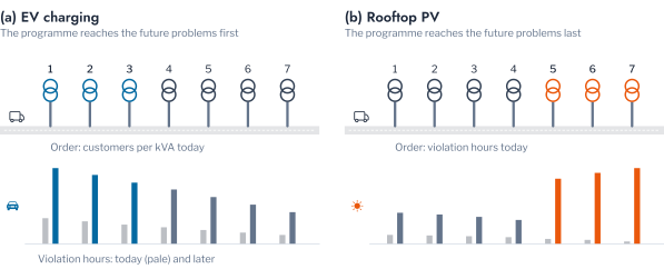
A reinforcement programme examines transformers in order, and the order is set before the adoption it guards against has arrived. The evaluation therefore ranks the 43 residential transformers of HPK11 by what is observable at 20% penetration in DSS-AU, and judges the order by the violation hours each transformer incurred at 80%. For PV, the relevance \(\mathrm{rel}_i\) of a transformer is its hours above \(\overline{v}\) at 80% PV and 20% EV penetration. For EV, it is its hours below 0.94 pu or above its rating at 80% EV and 20% PV penetration. Figure 8.1 illustrates why the two need not behave alike.
The record of DSS-AU shows the difference before any score is fitted (Figure 8.2). Under EV charging the transformers that were most loaded at 20% were largely those with the most violation hours at 80%. Under PV, 35 of the 43 transformers already exceeded \(\overline{v}\) at 20%, for a median of 183 hours among them, but the transformers with the most hours at 20% were not those with the most at 80%, because the hours grew at rates that differed between transformers.
Five scores were compared against a random order. Customers per kVA and today’s violation hours are the two heuristics a utility holds without a model, the latter counting hours above \(\overline{v}\) for PV and hours above 90% of the rating for EV. Three pointwise models, the five nearest transformers, a linear regression and gradient-boosted trees, were fitted to the later hours from all of today’s features, including the impedance of the connection points and the composition of each transformer’s customers, and scored each transformer when left out of the fit. A listwise ranker of the kind Chapter 1 described learns from many lists, and one network supplies a single list of 43 transformers, so the pointwise models are the learned scores of this chapter. The NDCG at 5 used five grades, the quintiles of the later hours, and Kendall’s \(\tau_b\) was computed on the hours themselves. Intervals were obtained from 1,000 bootstrap resamples of the transformers.
For EV the heuristics sufficed (Figure 8.3). Customers per kVA placed the five worst transformers first, with an NDCG at 5 of 1.000 and a \(\tau_b\) of 0.604, and today’s hours reached 0.963 and 0.562. The gradient-boosted trees reached the highest \(\tau_b\), 0.637, but its interval from 0.548 to 0.714 overlapped those of both heuristics. Charging adds load in proportion to the number of customers, so the transformer that is most heavily loaded per kVA today remains so at 80%. A utility preparing for electric vehicles can therefore order its transformers by customers per kVA, a quantity of its asset register, without fitting a model.
For PV the heuristics failed. Today’s hours above \(\overline{v}\) reached a \(\tau_b\) of only 0.196, and customers per kVA 0.053, no better than the random order at 0.048. The learned scores reached 0.504 to 0.573, with intervals that excluded both heuristics, and so recovered much of the later order that today’s hours missed. The NDCG at 5 was less informative. A random order reached 0.742, with an interval from 0.468 to 0.927 that contained every learned score, because, with 43 transformers in five grades, a random choice of five places often attains a high gain. The top of a single short list cannot separate the scores, and the order of the whole list is the more reliable criterion for a programme of this size.
Ranking by Today’s Events
Today’s hours count how long a transformer violates its limits, but not how, in one long afternoon or in many brief excursions, slightly or far beyond the limit. Part 5 described each violation event by its duration, its depth and its timing (Equation 4.17, Figure 4.7) and grouped the events of HPK11 into eight violation patterns. The same description characterises a transformer by its events today. For transformer \(j\) and kind \(\kappa\) of violation, with \(\mathcal{E}_{j\kappa}\) its events at 20% penetration, the severity is the summed excess integral,
\[ S_{j\kappa} = \sum_{e \in \mathcal{E}_{j\kappa}} I_e, \tag{8.1}\]
which weighs depth and duration together. Each transformer is further described, for each kind, by the number of its events, the mean of the features of Equation 4.17 over them, its longest and deepest event, and the number of days with an event and with one sustained for at least one and for at least two hours. It is also described by the share of its event hours in each violation pattern \(r\) of Part 5,
The violation patterns were refitted with the description, sample, seed and number of violation patterns of Part 5, and reproduced its eight violation patterns exactly. Because the hours ignore depth, the transformers were ranked both against their hours at 80% and against their severity at 80%, Equation 8.1 applied to the later events.
For EV charging, the severity of today’s events was the best order (Figure 8.4). It reached a \(\tau_b\) of 0.712 against the hours at 80%, with an interval from 0.627 to 0.796 that excluded today’s hours at 0.562, and 0.772 against the later severity. No learned score improved on it, and gradient-boosted trees on the events and assets together reached 0.662. The severity weighs the depth of today’s evening excursions, which the hours ignore, and the transformers whose excursions were deepest at 20% were those that violated most at 80%. For PV, today’s events contained little information on the later order. The severity reached 0.195, no more than the hours, the violation pattern shares 0.172 and trees on the event features 0.367, while trees on the events with the asset features reached 0.586, no more than trees on hours and assets at 0.575. The timing and depth of today’s over-voltage thus add nothing to the position of a transformer in the network, which accounts for its later order.
Onset and Severity of PV Violations
The failure of today’s history to order the transformers for PV has a cause in the data. At 20% penetration, one customer in five has an array, and the violations of a transformer reflect where those first adopters happen to connect more than how much it can host; at 80% almost every customer has one, and the structure of the network decides. Two quantities separate the questions a Distribution System Operator (DSO) asks. The hosting capacity of transformer \(j\) is the penetration at which its over-voltage first breaches the criterion,
\[ \mathrm{HC}_j = \min \bigl\{ p : D_j(p) \ge 87.6 \bigr\}, \tag{8.3}\]
interpolated linearly between the simulated levels, and states when a transformer will need action; the hours and the margin at 80% state how severe its violations will then be. Two scores that do not depend on the first adopters were added. The voltage sensitivity measured from today’s record is the slope \(\beta_j\) of the regression of the highest customer voltage on the power of the transformer over the midday half-hours,
\[ v_j^{\max}(t) = a_j + \beta_j P_j(t) + \epsilon_j(t), \tag{8.4}\]
expressed per customer as \(-\beta_j n_j\), since a transformer of many customers changes its total power more for the same export of each. The screening study is the mean highest voltage of the transformer’s customers with every customer adopting, from the labelled risk set.
Today’s history ordered the onset and not the severity (Figure 8.5). Today’s hours ordered the hosting capacity with a \(\tau_b\) of 0.919, and the hours at 80% with 0.196. The severity was ordered by the structure of the network: the number of customers supplied, a quantity of the asset register, reached 0.560 for the hours and 0.598 for the margin at 80%, as high as trees on all of today’s features at 0.575 and 0.555, followed by the screening study at 0.504 and the measured sensitivity at 0.415. The sensitivity also ordered the hosting capacity, at 0.542, and adding it to the trees raised their order of the hosting capacity from 0.770 to 0.798. A transformer of many customers carries more export at high adoption, and the measured sensitivity adds how strongly its voltage responds. For a programme that asks when each transformer will need action, today’s history suffices; for one that asks how severe the violations will become, the register and a measurement of sensitivity serve better than the history.
A Second Network
A ranking learned on one network serves a utility with many only if it transfers. DSS-US records 30 pole transformers of a SMART-DS feeder in Austin, Texas, under the same 25 scenarios, judged against ANSI C84.1 Range A, 0.95 to 1.05 pu. Few of its transformers violate a limit even at 80%, three above 1.05 pu under PV and six overloaded under EV charging, so that hours would give almost every transformer the same relevance. The US transformers were therefore ranked by their margin to the limit. With \(x_j(t)\) the highest customer voltage under PV, or the loading under EV charging, of transformer \(j\) at half-hour \(t\) of the year at 80%, the relevance is its 99th percentile,
\[ \mathrm{rel}_j = Q_{0.99}\bigl( \{ x_j(t) \}_t \bigr). \tag{8.5}\]
The scores used what both records hold, today’s hours of each violation, the 99th percentiles of the loading and of the highest voltage, and the rating, standardised within each network, so that a model fitted on HPK11 ranks the US transformers by their position relative to their own network.
The transfer held for EV charging and not for PV (Figure 8.6). Today’s peak loading ordered the later loading with a \(\tau_b\) of 0.591, and gradient-boosted trees fitted on HPK11 alone reached 0.652, with an interval from 0.526 to 0.769, against 0.416 for the same model fitted within DSS-US. For PV, today’s highest voltage reached 0.425, the best of any score, while the learned scores reached 0.214 to 0.320 within DSS-US and 0.260 from HPK11. On the US feeder the voltage margin today ordered the margin later. The hours of HPK11 could not show such an order, because 35 of its 43 transformers were already beyond the limit at 20%.
Learning to Rank Across Networks
The scores so far were pointwise, each fitted to the outcome of a transformer and ranking only as a consequence. Chapter 1 described rankers that learn the order itself, pairwise and listwise, and a single list cannot test them. Liu frames learning to rank at the level of queries [4]. A ranker \(f\) is judged by its mean loss over the \(n\) queries \(q\) of a training set,
\[ \hat R(f) = \frac{1}{n} \sum_{q=1}^{n} L(f; q), \tag{8.6}\]
and Lan and colleagues showed that this risk approaches its expectation at a rate of \(1/\sqrt{n}\), so that a listwise ranker generalises with the number of lists rather than of items [8]. A pointwise score is not thereby inferior. Cossock and Zhang bounded the ranking error of a list of \(m\) items by the regression error of the score that orders it,
\[ 1 - \mathrm{NDCG} \le \frac{1}{\mathrm{IDCG}} \Bigl( \sum_{i=1}^{m} w_i^2 \Bigr)^{1/2} \Bigl( \sum_{i=1}^{m} \bigl( f_i - \mathrm{rel}_i \bigr)^2 \Bigr)^{1/2}, \tag{8.7}\]
with the weights \(w_i\) of Equation 6.13, so that a score that estimates the relevance accurately also orders it well [9]. The bound is sufficient but not necessary, since a perfect order can come from a score with a large regression error.
Each network supplies several lists when each pair of a penetration today and a higher one later is taken as a query: today 20% or 40% of the technology, later 60% or 80%, four queries per technology on each network. The relevance is the margin of Equation 8.5, graded into quintiles within each list for the listwise ranker. LambdaMART [6], [10] and pointwise gradient-boosted trees learned from the four lists of one network and ranked those of the other, with the features of both records standardised within each list. Their orders were also combined with the margin today by reciprocal rank fusion, which scores item \(i\) by its ranks \(r_s(i)\) under the scores \(s\) being combined,
\[ \mathrm{RRF}(i) = \sum_{s} \frac{1}{60 + r_s(i)}, \tag{8.8}\]
and requires no training [11]. Hybrid search engines that retrieve context for language models merge their keyword and vector rankings in the same way.
No learned ranker improved on the margin today when it learned from the other network (Figure 8.7). For EV charging on HPK11, the margin today ordered the later loading with a mean \(\tau_b\) of 0.919 over the four queries, against 0.628 for the pointwise trees and 0.588 for LambdaMART learned on DSS-US; on DSS-US the four scores lay between 0.621 and 0.651. For PV, the margin today reached 0.322 on HPK11 and 0.538 on DSS-US, the learned rankers 0.182 to 0.321. LambdaMART fell below the pointwise trees in two of the four cases and exceeded them by at most 0.032 in the other two, as Equation 8.7 allows and as four training lists from one network provide few terms to the average of Equation 8.6. The fusion was never the worst score and stayed within 0.14 of the better of its two components, at 0.785 and 0.629 for EV and 0.337 and 0.400 for PV, a property of value to a utility that cannot determine in advance which score will transfer.
Ranking by Risk Under Uncertain Adoption
The rankings so far ordered the transformers by their outcome in one future. A DSO that plans maintenance or replacement for thousands of transformers ranks them instead by risk, the likelihood of a failure to meet a limit combined with its consequence [1], and the future in which the likelihood is assessed is itself uncertain. The scenarios of DSS-AU provide that uncertainty. With adoption of each technology at the planning horizon distributed over the levels \(x \in \{0, 0.2, \dots, 0.8\}\) with probabilities \(\pi(x)\), here proportional to a normal density centred at 0.4 with a standard deviation of 0.2, a scenario \(s\) of EV penetration \(e_s\) and PV penetration \(p_s\) has the probability
\[ w_s = \pi(e_s)\, \pi(p_s). \tag{8.9}\]
Thermal and voltage violations are ranked separately, since their mitigation measures differ, transformer replacement for the one and voltage management for the other, and since the violation patterns of Part 5 separate them. For a constraint \(c\), with \(D_{jc}(s)\) the hours of violation of transformer \(j\) in scenario \(s\), its likelihood is the probability of breaching the hosting criterion of Equation 4.1,
\[ P_{jc} = \sum_{s} w_s\, \mathbb{1}\bigl\{ D_{jc}(s) > 87.6 \bigr\}, \tag{8.10}\]
its expected hours of violation are
\[ H_{jc} = \sum_{s} w_s\, D_{jc}(s), \tag{8.11}\]
and its risk weighs them by the \(n_j\) customers it supplies, in customer-hours outside the limits,
\[ R_{jc} = n_j\, H_{jc}. \tag{8.12}\]
Figure 8.8 illustrates the likelihood as the probability of the futures that breach and the ranking by likelihood and consequence. A utility cannot simulate every transformer, so the likelihood was also learned from what is observable today. A classifier estimates the probability \(\hat p(\mathbf{x}_j, e, p)\) that a transformer with today’s observables \(\mathbf{x}_j\) breaches the criterion at penetrations \(e\) and \(p\), fitted on the scenarios beyond today of the other transformers, and the learned likelihood weighs it by Equation 8.9,
\[ \hat P_{jc} = \frac{\sum_{s \in \mathcal{S}} w_s\, \hat p(\mathbf{x}_j, e_s, p_s)}{\sum_{s \in \mathcal{S}} w_s}, \tag{8.13}\]
where \(\mathcal{S}\) is the set of scenarios beyond today.
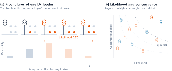
Under this distribution of adoption, the mean likelihood of breaching the criterion was 0.156 for overload and 0.797 for voltage on HPK11: most transformers will breach the voltage criterion, and the risk of each is therefore told apart by its expected hours and its customers rather than by its likelihood (Figure 8.9). The learned likelihood ordered the risk with a \(\tau_b\) of 0.726 for the thermal and 0.796 for the voltage constraint, with Brier scores of 0.078 and 0.065. For a programme that can inspect one transformer in five, the order of the learned likelihood captured 62.3% of the thermal risk and 41.0% of the voltage risk, against ceilings of 66.4% and 41.8% for the order of the risk itself (Figure 8.10). Customers per kVA captured 64.4% of the thermal risk but only 29.7% of the voltage risk, and today’s violation hours 60.7% and 24.6%. The learned likelihood thus served both programmes, whereas each heuristic served only the thermal one. Its probabilities did not transfer to DSS-US, whose transformers rarely breach the criterion: learned on HPK11, the classifier reached Brier scores of 0.336 and 0.889 there, so that a utility must calibrate the probabilities on its own network before it ranks by them.
Pitfall: a short list judged by its top
The NDCG at 5 is the measure of a ranking that matters to a programme that acts on its first five items, and it is the measure that learning to rank optimises. On a list of a few dozen transformers graded into five levels, however, a random order already attains a high gain, because a random choice of five places often holds items of high grade: on HPK11 a random order reached an NDCG at 5 of 0.742, with an interval that contained every learned score. A comparison of rankers by their gain at the top of one short list therefore cannot separate them, and the order of the whole list, by Kendall’s \(\tau_b\), or the gain over many lists, is the criterion that distinguishes a ranking from chance.
Ranking Live Violations for Operators
The recommendations of the preceding sections are made in planning, before the violations they address occur. During operation, violations begin while others are in progress, and an operator must determine which to address first. This is a ranking problem in the sense of Chapter 1. Each day of each penetration scenario of DSS-AU is a query in the query-level framework of learning to rank [4], and its list contains the violation events of that day, each represented as it is observed one hour after it began: its excess in its first two half-hours, its kind, the time and season of its start, the penetration scenario, and the rating and customers of its transformer. The relevance of an event is its final severity, the excess integral \(I_e\) of Part 5, which is unknown when the event is ranked (Figure 8.11). Events that end within their first hour are complete before they can be ranked and are excluded.
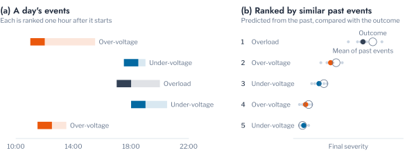
An event \(e\) is scored by the mean logarithmic severity of the \(k = 20\) past events nearest to it in the standardised features observed at one hour,
\[ \hat s_e = \frac{1}{k} \sum_{e' \in \mathcal{N}_k(e)} \log \bigl( 1 + I_{e'} \bigr), \tag{8.14}\]
which is the retrieval of Equation 6.3 applied to events, and by gradient-boosted trees fitted to the same target. Both are pointwise scores in the sense of Chapter 1, which order the events of a day through an estimate of the severity of each, and Equation 8.7 bounds the error of the ranking by the error of that estimate. Both are compared with the two quantities that an operator observes without a model, the current excess and the severity accumulated so far, and with a random order. The past events are those of the first half of each month and the days ranked those of the second half, so that no day contributes to both and events of the same day cannot inform one another, a form of leakage that would inflate the measured accuracy [12]. Each ranking is evaluated by the NDCG at 5 of Equation 6.15, the precision at 5 of Equation 6.11, and the share of the violation hours still to come that the five events ranked first account for, averaged over the days, with intervals from 500 bootstrap resamples of the days.
Scores learned from past events ranked the violations of each day more accurately than the quantities an operator observes directly (Figure 8.12). Over 2,331 days and 96,202 events, the gradient-boosted trees reached an NDCG at 5 of 0.962 and placed 81.0% of the five most severe events of a day among their first five, against 0.931 and 67.7% for the current excess and 0.916 and 62.1% for the severity so far. The nearest past events of Equation 8.14 reached 0.933 and 74.2%. The five events ranked first by the gradient-boosted trees accounted for 94.8% of the violation hours still to come among the five most severe events, against 86.1% for the current excess. On a typical day, an operator who attends first to the five events ranked highest by the model therefore attends to one more of the five most severe events than the current excess indicates.
Further Applications of Ranking on the Network
The two rankings of this chapter, of assets by an outcome that lies in the future and of events by a severity that is not yet known, apply wherever a distribution network operator must order more work than it can do at once. Three further problems take the same form.
The first is the order in which meters flagged as faulty are inspected. Part 7 assigns each meter a conformal p-value for each day, and the procedure of Benjamini and Hochberg controls the share of false flags among those inspected; the order of inspection within the flagged meters is a ranking whose relevance is the energy that a fault misrecords, which the size of the meter’s demand and the length of its anomalous run estimate. A pointwise score of that loss, as in Equation 8.7, orders the inspections, and the crews visit first the faults that cost most.
The second is the order in which ageing transformers are replaced. The ageing of a transformer’s insulation follows the depth and the duration of its overloads, which the integral of its events in Equation 8.1 measures, and a ranking by the expected ageing at the penetration a plan anticipates replaces a ranking by age alone, which ignores the loading that adoption adds.
The third is the order in which customers receive an offer of flexibility. Chapter 1 ranked the households of the Low Carbon London trial by their estimated response to a time-of-use tariff, and the same ranking, with the relevance the reduction of demand at the peak of a constrained transformer, orders an offer of managed charging or of a battery so that the first offers relieve the transformers that the ranking of this chapter places first.
Conclusion
This chapter ranked the transformers of HPK11 for the network of later years and the violations of each day for the operators who respond to them. Ranking transformers depended on the technology. For EV charging, customers per kVA today ordered the transformers as well as any learned score, so that a utility can rank them from its asset register. For PV, today’s violation hours contained little information on the later order, and pointwise models fitted to the features raised Kendall’s \(\tau_b\) from 0.196 to between 0.504 and 0.573. The severity of today’s events ordered the transformers for EV charging better than any other score, at 0.712, while for PV the events added nothing to the features of the network. Today’s history ordered the onset of PV violations, with a \(\tau_b\) of 0.919 against the hosting capacity, but not their severity at high adoption, which the number of customers supplied ordered at 0.560.
On a second network, a model fitted on HPK11 ordered the EV loading margins of 30 US transformers at 0.652. Learned across networks, neither pointwise trees nor LambdaMART improved on the margin today, and a reciprocal rank fusion of the two was the most robust order. Ranked by risk under uncertain adoption, separately for the thermal and the voltage constraint, a learned likelihood captured 62.3% of the thermal and 41.0% of the voltage risk when one transformer in five was inspected. During operation, violations ranked one hour after they began were ordered more accurately by models of past events than by the quantities an operator observes directly, with a precision at 5 of 0.81 against 0.68 for the current excess.
The ranking uses two networks, 43 transformers on HPK11 and 30 on DSS-US, and four lists on each, too few for a listwise ranker to show the advantage that many queries give it, and the adopters of each scenario are drawn at random, so that the first adopters of a real network, who may not be random, could order the onset differently. Chapter 4 turns from ordering the transformers to choosing the mitigation measure for each.
Exercises
- Replace the five grades of the
rankingcell with three and with ten. How do the NDCG at 5 of the random order and its interval in Figure 8.3 change, and which number of grades gives the narrowest intervals? - Rank the transformers for PV by the mean resistance of their connection points alone. How close does this single feature come to the learned scores of Figure 8.3?
- Rank the transformers of HPK11 by their margin, Equation 8.5, rather than by their hours. Does today’s highest voltage then order the later margins as it did on DSS-US?
- Increase the number of nearest past events in Equation 8.14 from 20 to 100. How do the NDCG at 5 and the precision at 5 of Figure 8.12 change, and why does a larger neighbourhood favour the long midday events over the brief evening ones?
- Rank the live events after their first half-hour rather than their first hour. What share of the advantage of the learned scores over the current excess remains?