Network Risk
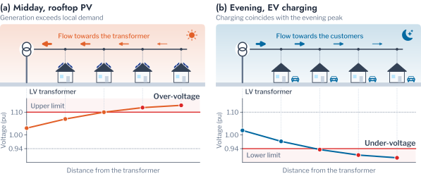
The operation of a Low Voltage (LV) network is bounded by two constraints. The voltage at every customer must remain within a statutory band, and the loading of every transformer must remain within its rating. Rooftop Photovoltaic (PV) and Electric Vehicle (EV) charging act on both, in opposite directions (Figure 4.1). Midday export from PV raises voltages along the feeder. Where it exceeds local demand by a wide margin, it reverses the flow through the transformer and overloads it. Evening charging, by contrast, adds demand at the hour of the daily peak and lowers voltages at the ends of long feeders. A Distribution System Operator (DSO) must therefore decide, for each transformer, which mitigation measure it needs and in what order to apply them. The measures are voltage control, which includes reactive power control and curtailment of export, and additional capacity [1], [2].
The decision rests on the records that a DSO holds, which are the smart-meter time series of its customers and the record of limit violations on its transformers. Chapter 3 grouped households by the shape of their demand, on the premise that households which use energy at similar times load the network similarly. This chapter applies the clustering workflow of Chapters 1 to 3 to the second kind of record, the violations, and tests that premise against the decision on a real network. The test is possible because the 342 AusNet households form the demand pool of four published network models.1 Each model joins a medium-voltage and a low-voltage network. The households that were clustered can therefore also be placed on a network and simulated. The urban network HPK11, with 5,274 residential customers on 43 transformers, is used throughout.
Each section pairs the power theory that defines a limit with the clustering step that organises its violations and with the decision that the result informs. Three questions structure the work of this chapter. The first is how violations develop as adoption grows and whether they fall into kinds that call for different measures. The second is which transformer needs which measure, and from what penetration. The third is how much the load pattern of a household adds to either answer.
Hosting Capacity
The established frame for assessing Distributed Energy Resources (DER) on distribution networks is hosting capacity [3], [4], [5]. It is the amount of generation or demand that a network can accommodate before a performance index, such as the time a voltage spends outside its band, exceeds its limit. The outcome depends on which customers adopt and on what they consume. Probabilistic impact assessments therefore sample household demand profiles and the locations of adoption, and report the share of feeders that remain within their limits as penetration grows [6]. Recent work estimates hosting capacity from smart-meter data and voltage sensitivities in place of repeated power-flow studies [7], [8], [9].
For a transformer \(j\) at a penetration \(p\), the criterion used here is that the time beyond a limit stays within a small share of the year. Let \(D_j(p)\) be the total duration, in hours, of the events of one kind at the transformer over a period of \(T\) hours. The transformer hosts the penetration when
\[ D_j(p) \le \varepsilon T, \qquad \varepsilon = 0.01, \quad T = 8{,}760 \text{ h}, \tag{4.1}\]
that is, when the limit is breached for at most 87.6 hours in the year. The share of 1% is a planning criterion of hosting studies and not a clause of EN 50160 or of AS 61000.3.100, which state their own percentiles. It is stricter than the 95% of weekly intervals that EN 50160 requires within the band. The largest adoption that every transformer and every limit accept is the hosting capacity of the network. The decision problem of the operator is to find it for the penetration that the plan anticipates.
The measures differ by constraint: curtailment of active power or reactive power control addresses the over-voltage of PV export [10], [11], and coordinated charging addresses the evening demand of charging [12]. Two gaps follow for the use of clustering. Hosting studies summarise violations as shares of time or of feeders within limits. These shares do not distinguish a long midday excursion from many brief evening ones, although the two call for different mitigation measures. Load-profile segmentation has been assessed by internal indices and by the correspondence of its clusters with household characteristics [13], [14], [15]. It has seldom been assessed by the network outcomes that it is proposed to inform. This chapter addresses both gaps in three steps. It clusters the violations into violation patterns that point to a mitigation measure, and it clusters the transformers by the violations they incur as adoption grows. Finally, it measures how much of the risk of each customer its load pattern carries. Chapter 5 evaluates the uses of clustering that the result points to.
Remark: why generation raises voltage and charging lowers it
A feeder delivers power from the transformer to the customers, and voltage falls along the direction of flow. A customer that exports reverses the flow on its own cable, so its voltage rises above that at the transformer. A charger adds to the flow and deepens the fall. The effect grows with the resistance of the path.
Network Model
A low-voltage network is a radial tree rooted at its distribution transformer, and its voltages follow from the demand of its customers through the laws of alternating-current circuits. For bus \(i\) with voltage magnitude \(V_i\) and angle \(\theta_i\), and a bus admittance matrix \(\mathbf{Y} = \mathbf{G} + j\mathbf{B}\), the injected active and reactive power are
\[ P_i = V_i \sum_{k} V_k \bigl( G_{ik} \cos\theta_{ik} + B_{ik} \sin\theta_{ik} \bigr), \tag{4.2}\]
\[ Q_i = V_i \sum_{k} V_k \bigl( G_{ik} \sin\theta_{ik} - B_{ik} \cos\theta_{ik} \bigr), \tag{4.3}\]
with \(\theta_{ik} = \theta_i - \theta_k\). These are the equations that the power-flow solver of OpenDSS solves for every half-hour, by the iterative methods of Newton and of the compensation-based algorithms for radial networks [16], [17]. They are nonlinear, so the effect of one customer on the voltage of another cannot be written down directly.
On a radial network the branch flow equations give a linear approximation that explains the behaviour of the voltage [18], [19], [20]. Consider the branch from bus \(i\) to bus \(j\) with resistance \(r_{ij}\) and reactance \(x_{ij}\). Let \(P_{ij}\) and \(Q_{ij}\) be the active and reactive power that it carries towards the customers, and let \(v = V^2\). Neglecting losses, the squared voltage falls along the branch by
\[ v_j = v_i - 2\bigl( r_{ij} P_{ij} + x_{ij} Q_{ij} \bigr), \tag{4.4}\]
and the power \(P_{ij}\) carried by a branch is the demand at its far bus plus the power carried by the branches beyond it in the tree. For a customer at the end of a feeder with source voltage \(V_0\), the two relations reduce to the voltage change
\[ \Delta V \approx \frac{R P + X Q}{V_0}, \qquad R = \sum_{\ell \in \text{path}} r_\ell, \tag{4.5}\]
where \(P\) and \(Q\) are the power that the customer draws, negative for an export. \(R\) and \(X\) are the resistance and reactance of the path to the transformer [1], [21], [22]. The approximation follows from \(V_0 - V = Z I\) with \(I = (P - jQ)^{*}/V^{*}\) and \(V \approx V_0\). On low-voltage cables the resistance exceeds the reactance, so active power dominates the rise. The resistance of the path, which this chapter calls the electrical distance of the customer, sets how far its own export moves its voltage.
The power that a customer injects is its generation less its demand and its charging,
\[ p_i(t) = p_i^{\text{PV}}(t) - p_i^{\text{load}}(t) - p_i^{\text{EV}}(t), \tag{4.6}\]
where the output of an array follows the irradiance, derated for the temperature of the cells [23]. The inverters follow the volt-VAr and volt-watt characteristics of AS/NZS 4777.2, which reduce the active and reactive power as the voltage rises [10]. The transformer carries the sum of the injections of its customers, so its loading relative to its rating \(S_{\text{rated}}\) is
\[ \lambda(t) = \frac{\sqrt{\bigl(\sum_i p_i(t)\bigr)^2 + \bigl(\sum_i q_i(t)\bigr)^2}}{S_{\text{rated}}}, \tag{4.7}\]
which exceeds one when the transformer is overloaded by demand. It also exceeds one when the customers export more than its rating, since a reverse flow overloads the transformer in the same way. The statutory limits are a voltage band and the rating,
\[ 0.94 \le V_i(t) \le 1.10 \text{ pu}, \qquad \lambda(t) \le 1, \tag{4.8}\]
the band of AS 61000.3.100 on a base of 230 V. The voltage limit is local to each customer and depends on its electrical distance, whereas the loading limit depends on the sum over all customers. A single distant exporter can therefore breach the voltage limit long before the sum of the exports approaches the rating. This predicts that over-voltage binds before overload, and Response to Penetration tests the prediction against the simulated records.
Pitfall: applying the voltage-rise formula where it does not hold
The relation of Equation 7.1 neglects losses and assumes \(V \approx V_0\). It misleads for a customer whose own export is large enough to reverse the flow at its bus. It also misleads on a network with active reactive power control, where the reactive term changes sign. Use it to rank customers and to predict which limit binds, and solve the power flow for the voltage itself.
Scenarios and Placement
The network analyses use HPK11, the urban network of Hampton Park, Victoria. Its definition is rebuilt from the published workbook as an OpenDSS model of the 22 kV feeder and the 44 LV transformers of 200 to 1,000 kVA beneath it. A pseudo LV network extends to every customer. One transformer supplies no residential customer and records no customer voltage, so the analyses at the level of the transformer concern the other 43. Each of the 5,274 residential customers is assigned the measured load profile of one of the 342 AusNet households, drawn with replacement under a fixed seed. Each household therefore appears at about fifteen locations, and the load pattern of every customer is known.
Two sources provide the network outcomes of the chapter. The DSS-AU dataset records every half-hour of 2019 for each LV transformer under 25 scenarios. PV and EV penetration each range from 0 to 80% of customers in steps of 20. Arrays of \(6.6 \pm 2.0\) kWp follow measured irradiance with temperature derating and the AS/NZS 4777.2 characteristics, and chargers follow recorded charging sessions. Each record holds the loading of the transformer relative to its rating and the lowest and highest voltage among its own customers. Where a question requires control over which customers adopt, or over the load profile assigned to each customer, the same model is solved directly over a clear day. Every customer is equipped with a 5 kWp array and a 7.36 kW charger, and the outcome of every customer is stored. The solver records a step that does not converge as a missing value. Of the 19.3 million records, the only missing values belong to the transformer that supplies no residential customer, so every step of the 43 transformers converged in all 25 scenarios.
The sampling of households has a consequence for every statistic of the chapter. Suppose that each of \(n\) households is drawn \(m\) times, and that the outcomes of copies of one household have intraclass correlation \(\rho\). The variance of a mean over the \(nm\) customers is
\[ \operatorname{Var}(\bar y) = \frac{\sigma^2}{nm} \bigl[ 1 + (m - 1)\rho \bigr], \tag{4.9}\]
so that the effective number of independent customers is \(nm / [1 + (m - 1)\rho]\) [24]. Here \(m \approx 15.4\), and the intraclass correlation is the share of the variance that lies between households, which What Load Patterns Add measures. It is 0.68 for the contribution of a customer to the peak, an outcome that the household decides, so the effective number of customers is about 490 and not 5,274. It is 0.003 for the worst voltage, which the point of connection decides, so the 5,274 customers are nearly independent for that outcome. A significance statement that counts every customer as independent is therefore too confident for the first outcome and acceptable for the second. The shares of variance are read against their chance level and not against zero.
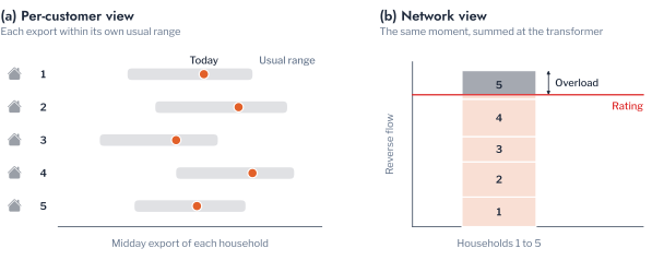
Outcomes are recorded at the transformer, and not at each customer, because a violation arises from the coincidence of ordinary demands on one transformer. The variance of the demand \(D\) of \(N\) customers is
\[ \operatorname{Var}(D) = \sum_{i} \operatorname{Var}(x_i) + \sum_{i \ne k} \operatorname{Cov}(x_i, x_k), \tag{4.10}\]
so that the diversity among customers, which keeps the covariance low, is what keeps the peak of the transformer below the sum of the peaks of its customers [25]. Figure 5.4 illustrates this for export: the midday export of each household lies within its own usual range, and only their sum at the transformer exceeds the rating.
Remark: what crosses to the planning team
A hosting study needs the violation records of the transformers and the model of the network, and it does not need the household readings. The records can be computed by the metering team from the readings and passed on as events. The half-hourly profile of each household, and the behaviour it reveals, then stays with the team that holds the meters.
Violation Events
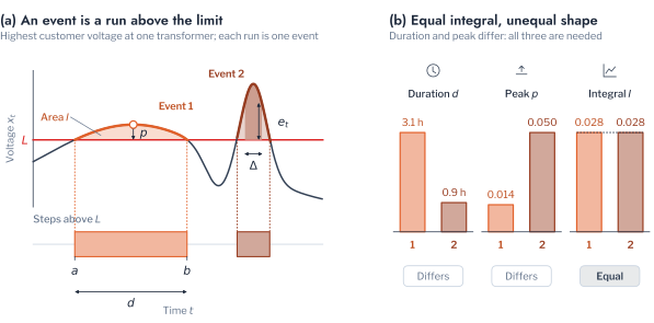
Even at the level of the transformer, a record of 19.3 million half-hours requires a summary. A share of half-hours beyond a limit indicates how often the limit is breached. It does not show whether the breaches form one long afternoon or many brief excursions, which call for different mitigation measures. The record is therefore summarised as events, the excursions of a random process beyond a level that Rice analysed [26], [27]. For a series \(x_t\) at a transformer and an upper limit \(L\), the excess is
\[ e_t = x_t - L, \tag{4.11}\]
and \(e_t = L - x_t\) for a lower limit. An event is a maximal run of consecutive steps \(a \le t \le b\) with \(e_t > 0\), characterised by its peak excess \(\max_t e_t\), by its duration
\[ d = (b - a + 1)\,\Delta, \tag{4.12}\]
where \(\Delta\) is half an hour, and by its integral
\[ I = \Delta \sum_{t=a}^{b} e_t, \tag{4.13}\]
which weighs depth and duration together. The integral is the quantity that the physics of the equipment follows. The ageing of the insulation of a transformer accelerates with the hot-spot temperature \(\theta_H\) by the factor2
\[ F_{AA}(t) = \exp\!\left( \frac{15000}{383} - \frac{15000}{\theta_H(t) + 273} \right), \tag{4.14}\]
and \(\theta_H\) rises with the depth and the duration of an overload. The equivalent ageing over a period is the integral of \(F_{AA}\), a closer measure of the damage than the number of half-hours above the rating [28], [29].
Four kinds of event are extracted, and two of them concern voltage. Over-voltage and under-voltage occur when the highest or lowest customer voltage leaves the AS 61000.3.100 band of 0.94 to 1.10 pu. Overload occurs when the apparent power exceeds the nameplate rating, and high loading when it exceeds 90% of the rating, the early warning of an overload. The year yielded 292,041 events across the 25 scenarios. Figure 4.3 illustrates the definition and shows why duration, peak excess and integral are all required, since a long, shallow event and a brief, deep one can enclose the same area.
Response to Penetration
With violations defined as events, the response of the network to DER can be described in terms that bear directly on decisions. This section characterises how violations develop as penetration grows, which transformers reach their limits first, and when the violations occur.
Frequency, Duration and Depth of Violations
Figure 4.4 shows the share of the time of 2019 that each kind of violation occupied across the 25 scenarios. The share is the total duration divided by the 376,680 transformer-hours of the 43 transformers. It can therefore be compared with the criterion of 1% of the time for one transformer. The two technologies stressed the network along different constraints. Over-voltage depended almost entirely on the generation of the arrays. It was absent without PV, occupied 2.33% of the time at 20% PV and rose to 12.36% at 80%. EV adoption reduced it only slightly, to 11.65% at 80% of both. Under-voltage depended on EV adoption, rising from 0.006% of the time without DER to 0.28% at 80% EV. Overload took a different course with each technology. It was negligible with PV up to 40%, at 0.10%. It then grew steeply to 2.21% at 60% and 7.72% at 80%, as exports began to exceed the rating of the transformers. With EV alone it reached only 0.25% at 80%.
For planning, the asymmetry means that the two technologies call for different studies. A transformer facing PV adoption must be assessed for voltage first and for reverse loading as adoption passes 40%. A transformer facing EV adoption must be assessed for loading and under-voltage in the evening. An assessment of one technology says little about the other.
The events also differed in character, as the two 80% scenarios show. With PV at 80%, the 11,606 over-voltage events lasted 4.01 hours on average and up to 9.00 hours, but rose at most 0.05 pu above the limit. The 7,020 overloads lasted 4.14 hours on average and reached 1.15 pu beyond the rating, a loading of 2.15 times nameplate. With EVs at 80%, events were shorter, with mean durations of 1.19 hours for the 876 under-voltage events and 1.63 hours for the 565 overloads. Under-voltage reached 0.09 pu below the band and overload 0.69 pu beyond the rating. A violation of voltage is long and shallow, so it is a matter of how long a customer is exposed. A violation of loading is deep, so it is a matter of how far the equipment is stressed. Both properties are needed to choose a mitigation measure, and a count of half-hours beyond a limit contains neither.
Hosting Thresholds
These totals aggregate over transformers that differ widely in their exposure. The criterion of Equation 4.1 judges each transformer separately, taking the time beyond a limit within the year and accepting the penetration when it is at most 87.6 hours. The order in which the limits bind follows from the voltage rise along a feeder. By Equation 7.1 a single distant customer can exceed the voltage limit long before the sum of the exports approaches the rating, which predicts that over-voltage binds before overload. Figure 4.5 reports the share of transformers that meet the criterion, and the data confirm the prediction.
Over-voltage was the binding constraint by a wide margin. At 20% PV only 41.9% of the 43 transformers remained within the criterion, with a median of 146.5 hours of over-voltage. At 40% only 7.0% did, with a median of 565.5 hours, and by 80% none did. PV-driven overload became binding later, as 95.3% of the transformers hosted 40% PV, 60.5% hosted 60% and 16.3% hosted 80%. EV adoption was accommodated more readily: at 80% EV, 90.7% of the transformers remained within the criterion for under-voltage and 95.3% for overload. The first limit to reach a transformer is therefore voltage under PV and under-voltage under EV, so hosting studies should test them first. A feeder model with loading alone would approve adoption that the voltage limit refuses.
Hosting thresholds state how much violation a transformer incurs but not when it occurs, which determines both the mitigation measure and the period that a study must simulate. The event record places each violation in time. PV-driven over-voltage occupied the hours from 08:00 to 16:00, with 90.7% of the transformer-hours between 09:00 and 15:00. It followed irradiance through the year, from 7,268 transformer-hours in January to 994 in July. EV-driven violations occupied the hours from 16:00 to 22:00, with 93.5% of the transformer-hours there and the largest number at 19:00. A study of the PV problem needs the summer months and the midday hours, and a study of the EV problem the evening of the heaviest day.
Pitfall: assessing a transformer at the adoption of today
A transformer that meets the criterion at the current penetration may fail it on a different constraint at a higher one. Reverse-flow overload was nearly absent below 40% PV and became large at 80%. An assessment at 20% therefore reports a voltage problem and misses the thermal problem, which needs a different measure. Evaluate the criterion at every penetration up to the level that the plan anticipates.
Clustering Design
This chapter applies the clustering workflow of Chapters 1 to 3 to the records of a distribution network, and it adds nothing to the methods themselves. Chapter 3 chose a representation, a scaling, a reduction and an algorithm. Chapter 2 chose the number of groups and verified it against structureless data. Chapter 3 then checked the result against structure that the design had not seen. Figure 4.6 lists the steps for the two units that are clustered here. What is new is the unit, the representation that describes it and the outside check, and this section states those three.
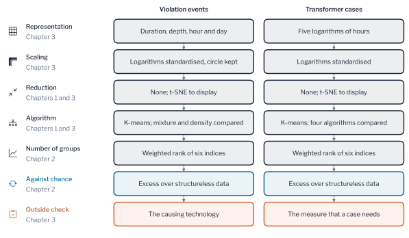
The chapter clusters two units, the events and the transformer cases. An event is a maximal run beyond a limit (Violation Events), and it is described by the six features of Equation 4.17. The two logarithms are standardised to zero mean and unit variance. The sine and the cosine of the hour and of the day keep the geometry of the unit circle, as Chapter 3 prescribes for features on a circle. A transformer case \(c = (j, p, q)\) is transformer \(j\) at a PV penetration \(p\) and an EV penetration \(q\). Let \(D_{c,m}\) be the hours of violation of the case in pattern \(m\), \(U_c\) its hours of under-voltage and \(N_c\) its number of events in the year. The case is described by
\[ \boldsymbol{\psi}_c = \bigl( \log(1 + D_{c,1}),\ \log(1 + D_{c,2}),\ \log(1 + D_{c,3}),\ \log(1 + U_c),\ \log(1 + N_c) \bigr), \tag{4.15}\]
where the logarithm compresses hours that range from half an hour to about 1,700 hours in a pattern, a ratio of more than three thousand. Adding one before the logarithm places a case without violation at the origin. The representation fixes what a group can mean, since two units are close only if they agree on the properties that describe them. Its choice therefore matters more than the choice of algorithm, as Chapter 3 showed for households. Violation Patterns compares four representations of a violation against a structure that none of them uses.
The outside check is the decision that the clustering is meant to inform. A violation pattern points to a mitigation measure. Pattern 1, the long midday over-voltage, is answered by voltage control. Pattern 2, the deep overload of reverse flow, is answered by capacity, whereas pattern 3, the brief excursion, contributes little exposure and needs neither. A transformer case \(c\) needs a measure \(r\) when the hours of the patterns that \(r\) answers exceed the criterion of Equation 4.1,
\[ \mathcal{R}_c = \bigl\{ r : D_{c,r} > \varepsilon T \bigr\}, \tag{4.16}\]
where \(D_{c,r}\) is the total duration of the events in those patterns. The set is empty when the case meets the criterion, and its elements are the measures that the operator must schedule. A partition is useful when its groups are homogeneous in this set. Their agreement is the purity of Equation 2.6, with the sets of measures as the known grouping. It is the accuracy of the decision map that assigns to each group its commonest set of measures. It must be read against groupings that use no clustering, which are the adoption rate alone and random groups of the same sizes. The set \(\mathcal{R}_c\) is a function of the same hours that describe a case. Purity therefore shows what a partition retains of the decision and is not an independent validation.
Violation Patterns
The four kinds of event defined in Violation Events classify violations by the limit they breach, yet Response to Penetration showed that violations of one kind differ in duration, depth and timing. These properties determine the mitigation measure: a long midday over-voltage calls for reactive power control or a curtailment of export [10], [11], and a brief evening excursion for coordinated charging [12]. Clustering the events themselves recovers this structure without prior labels, as the design of Clustering Design states. This section applies the workflow of Figure 4.6 to the events. The representation is set in Event Features and the algorithm in Number of Patterns. The outside check follows in Description of Patterns and in Events and Time Series.
Event Features
Each event is described by
\[ \boldsymbol{\phi} = \left( \log d,\ \log (e^{*} + \epsilon),\ \sin \tfrac{2\pi h}{24},\ \cos \tfrac{2\pi h}{24},\ \sin \tfrac{2\pi y}{365},\ \cos \tfrac{2\pi y}{365} \right), \tag{4.17}\]
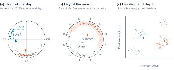
where \(d\) is its duration, \(e^{*}\) its peak excess, \(h\) the hour of its midpoint and \(y\) its day of the year. The constant \(\epsilon = 10^{-4}\) pu keeps the logarithm finite for an event that only grazes its limit (Figure 4.7). Time sits on a circle because 23:00 and 01:00 are close. The Euclidean distance between two points of the unit circle is the chord \(2\sin(\delta/2)\) of the angle \(\delta\) between them [30]. Only the two logarithms are standardised to zero mean and unit variance. Scaling the sine and the cosine by their own spreads would distort the chord whenever the events cluster at one time of day, as the midday events do here.
The two logarithms describe how long and how deep a violation is, which determines the equipment that must answer it. The sine and the cosine of the hour describe the cause, since generation acts at midday and charging in the evening. Those of the day of the year describe the season. A violation of one kind that is long and shallow differs in the measure that it needs from one that is brief and deep. The features therefore separate violations by the measure that they call for and not by the limit that they breach.
Number of Patterns
The algorithms of Chapters 1 and 3 are compared on the events. K-means assumes compact groups of similar spread, which is adequate when a group is a kind of event with one typical duration and depth [31]. The Gaussian mixture allows groups of unequal spread and gives each event a probability of membership, and a density method needs no number of groups [32]. The number of groups follows Chapter 2, by the weighted rank of six indices and the verification against structureless data, on a sample of 3,000 of the 221,070 events.
The weighted rank chose two groups, with a score of 8.40 against 7.43 for four groups and 6.97 for three. The verification kept two, but with a mean excess of 0.006 over structureless data, which is no better than the reproducibility of noise (Figure 4.8). Three groups had a mean excess of 0.193 and passed all three checks, as did four groups at 0.037 and nine to eleven groups at 0.083 to 0.188. Five to seven groups fell below chance, at excesses of \(-0.209\), \(-0.309\) and \(-0.148\). The excess of two groups is indistinguishable from noise. As Chapter 3 did for the AusNet households, the chapter therefore takes the second rule, the passing number with the largest excess, which is three. The finer partitions of nine to eleven groups are also supported by the data, and they would divide the brief events further. They rank lower on the six indices, and three patterns already separate the mitigation measures below.
Remark: the assumptions of the algorithm decide the number of groups
Four of five algorithms ranked two groups first, and the mixture ranked six, because it fits the spread of each group and the events do not have equal spread. A density method set 36.4% of the events aside as noise. The number of patterns is a property of the data and of the assumption together, which is why it is verified against chance.
The algorithms also agree on the partition only partly. At three groups the adjusted Rand index of k-means with Ward linkage was 0.65, with the mixture 0.46, with mini-batch k-means 0.42 and with BIRCH 0.34. The patterns are therefore the structure that k-means assumes, and a utility that adopts them should confirm that its measures do not rest on the boundary between them.
Description of Patterns
Figure 4.9 describes the three patterns in order of total duration. Pattern 1 holds 111,668 events and 69.0% of the 745,969.5 hours of violation. It is the long over-voltage of midday, with a mean duration of 4.61 hours and a median excess of 0.02 pu. Of its events 96% are over-voltage and 75% fall in the summer half of the year. It is answered by reactive power control or curtailment. Pattern 2 holds 38,745 events and 22.3% of the hours. It is the deep overload of reverse flow, with a mean duration of 4.29 hours and a median excess of 0.26 pu. Every event is an overload, centred at 12:15 and under high PV. It calls for a larger transformer or a limit on export, which voltage control does not supply. Pattern 3 holds 70,657 events and 8.8% of the hours. It is the brief excursion, with a mean duration of 0.93 hours and a median excess below 0.005 pu. It is of every kind, 81% over-voltage and 8% under-voltage, and it contributes little to the exposure of any transformer.
The three patterns therefore cut across the limit types in the way that matters for operation. Overload and over-voltage each appear in a long pattern and in the brief one, and the long overload needs a different measure from the long over-voltage. The evening violations of charging are too few to form a pattern of their own at three groups. There are 6,842 under-voltage events against 164,386 over-voltage events, and they fall into the brief pattern.
The patterns also differ in the technology that produces them (Figure 4.10). The events of pattern 1 occurred at a mean PV penetration of 60%, and 71% of them at 60% or more. The events of pattern 2 occurred at a mean of 73%, and 96% of them at 60% or more. Pattern 3 had a mean of 54% PV and 45% EV penetration, and it had the largest share of events without PV, 2.4% against 0.3% and 1.3%. The reverse-flow overload is therefore a phenomenon of high PV adoption, whereas the brief pattern is spread over both technologies.
The mean daily profile of each pattern shows the cause (Figure 4.11). On the days of pattern 1 the highest customer voltage averaged 1.114 pu at noon, above the limit of 1.10 pu. The loading of the transformer was 0.84 of its rating. On the days of pattern 2 the voltage averaged 1.117 pu and the loading was 1.25 times the rating at noon. The mean day of the reverse-flow overload therefore exceeds the rating as well as the limit. The days of pattern 3 peaked at 1.099 pu and a loading of 0.58, close to the limit and well below the rating. The three patterns therefore peak at the same hour and differ in level. The features of Equation 4.17 include the depth and the duration of an event for this reason, and not only its time.
Figure 4.12 places a sample of the events of each pattern on the features, and Figure 4.13 shows how the patterns emerged as penetration grew. Without DER the three patterns occupied only 0.002%, 0.009% and 0.006% of the time. PV at 20% brought pattern 1 to 1.88% of the time, and at 40% to 5.90%, while pattern 2 was still at 0.06%. Pattern 2 then grew to 2.00% at 60% and 7.40% at 80%. The dominant measure therefore changes as adoption passes 40%, which is the content of the pitfall of the previous section. Under EV the three patterns grew together, to 0.12%, 0.21% and 0.19% of the time at 80%.
The assignment can be checked against the record that produced it. Figure 4.14 shows one week of the transformer with the most over-voltage hours, with each violation shaded by its pattern. The long midday over-voltage of January falls in pattern 1 on every clear day, and the brief excursions of a cloudy day fall in pattern 3. Each shaded block can thus be read against the voltage that caused it.
Events and Time Series
The patterns describe events, but an operator also holds the time series from which the events were cut, and clustering applies to both. The design comparison of Chapter 3 settles which description to trust. The same transformers are described in four ways, and the groups are scored against a structure that no description uses, the technology that causes the violation: PV only, EV only or both, each at 80% penetration, with 600 units of each. Agreement is measured by the adjusted Rand index and the normalised mutual information of Chapter 2. The designs are compared over ten seeds by the paired test of Chapter 3.
The events are described by the features of Equation 4.17. The days with a violation are described by the 48 half-hours of the highest customer voltage, the lowest customer voltage and the loading, in two forms. The shape scales each channel to its own range within the day, which removes the level as the peak normalisation of Chapter 3 does. The profile keeps the level, with each column standardised. The fourth description gives each event the profile of the day on which it occurs, with the two blocks weighted to equal total variance. Each description is reduced by t-SNE (Equation 1.14), as Chapter 3 recommends, except the profile that keeps the level, which is clustered directly. All are grouped into three by k-means over ten seeds.
The profile that keeps the level recovered the technology best, with an adjusted Rand index of 0.542. The shape followed at 0.509, the events combined with the profile at 0.478 and the events alone at 0.455 (Figure 4.15). The normalised mutual information ordered the descriptions in the same way, from 0.586 to 0.486. A value of one means that the groups are the technologies, and a value near zero that they are unrelated to them. Every description therefore recovers about half of the structure. The level matters here because PV raises the voltage and EV charging lowers it, whereas in Chapter 3 the level hid the minority group that the shape revealed. Which representation wins therefore depends on the structure that the decision needs. The lesson of Chapter 3 holds in the form that the representation matters more than the scaler or the reduction.
Combining the two did not help beyond the better single description. Adding the profile to the events raised the index by 0.023 over the events alone and lowered it by 0.063 against the profile alone. The ten seeds gave identical scores to within 0.001, so the Wilcoxon \(p\)-value of 0.002 is the smallest that ten pairs allow, and the differences themselves are the evidence. The events kept 0.67 of the ten nearest neighbours after reduction, against 0.32 for the shape and 0.47 for the combination. The six numbers of an event therefore preserve their neighbourhoods best. The verification against structureless data supported five groups for the events at an excess of 0.265. It supported two for the shape at 0.023, which is no better than noise. An operator with complete daily records can therefore identify the technology of a violation best from the profile that keeps the level. An operator with events alone loses about 0.09 of agreement. It gains a description of six numbers that states the duration and depth of each violation, on which the measure depends.
Transformer Cases
The patterns describe the violations of the network as a whole, whereas the operator decides about transformers, and a transformer behaves differently as adoption grows. Each transformer at one combination of PV and EV penetration is therefore treated as a separate unit, a transformer case. The 43 transformers of HPK11 at 25 combinations give 1,075 cases, and the 30 transformers of DSS-US give 750. Clustering the cases asks whether transformers share a trajectory of exposure, and whether that trajectory is set by the rate of adoption or by the transformer itself. The workflow of Figure 4.6 applies unchanged to the cases. Case Groups chooses and verifies the groups and checks them against the measure that a case needs, and Rate and Transformer asks what the groups reflect.
Case Groups
A case is described by the hours of violation in each of the three patterns, the hours of under-voltage and the number of events in the year. Each quantity is taken on a logarithmic scale, so that a case without violation is a point at the origin and not a missing value. The number of groups follows the procedure of Chapter 3, with the weighted rank of six indices and the verification of Equation 2.27. On HPK11 the rank and the verification agreed on four groups, with a mean excess of 0.328 over structureless data. An excess of 0.33 in the sense of Equation 2.18 shows that the four groups are reproducible well beyond chance. The two patterns of events that the gate supported earlier reached an excess of only 0.006.
Figure 4.16 shows the cases themselves in two dimensions, coloured and numbered by group. Figure 4.17 shows the mean group of the transformers at each rate and how they move between groups as PV penetration rises. Figure 4.18 describes the groups, and Figure 4.19 gives the rates of adoption of their cases.
The groups form an ordered scale of exposure that rises with the rate of adoption. Group 1 holds 266 cases at a mean of 8% PV, with almost no violation and five events in the year. Group 2 holds 376 cases at a mean of 45% PV, with 504 hours of the long midday over-voltage, which calls for voltage control. Group 3 holds 207 cases at a mean of 63% EV penetration, with 560 hours of over-voltage, 175 hours of reverse-flow overload and 31 hours of under-voltage. Group 4 holds 226 cases at a mean of 72% PV, with 924 hours of over-voltage and 570 hours of reverse-flow overload, so it needs both measures. The groups are therefore stages of exposure and not kinds of transformer, and each stage names the measures that the transformers in it need.
The mean daily profile of each group completes the description (Figure 4.20). Group 1 stayed within the band, with a highest customer voltage of 1.078 pu and a loading of 0.38 of the rating. Group 2 reached 1.095 pu at noon, just below the limit on average, with a loading peak of 0.38 in the evening. This is the profile of a transformer that needs voltage control. Group 3 reached 1.092 pu at noon and a loading of 0.56 in the evening, the profile of charging added to generation. Group 4 reached 1.102 pu and a loading of 0.87 at noon. It is the only group whose average day exceeds the limit. Its loading peak has moved from the evening to midday, which is the mark of reverse flow.
The groups also carry information about the decision. Of the 1,075 cases, 449 needed voltage control alone, 257 needed both measures, 2 needed capacity alone and 367 needed none. The purity of Equation 2.6 for the four groups was 0.84. It was 0.75 for groups formed by the adoption rate alone and for the 25 cells of PV and EV rate. It was 0.52 for the 43 transformers and 0.42 for random groups of the same sizes. The adjusted Rand index with the set of measures was 0.54 for the groups, against 0.32 for the adoption rate and 0.07 for the cells of rate. The groups therefore retain more of the decision than the adoption rate does. The hours of violation in each pattern show which transformers have reached which stage at a given rate. On DSS-US no case needed either measure, so every grouping reaches a purity of one and the comparison carries no information there.
Pitfall: scoring a partition on the quantities that built it
A partition scored against a quantity computed from its own features appears more accurate than it is. The measures that a case needs are a function of the hours that describe the case, so purity shows what the partition retains and does not predict. Score a partition against structure that no step of its design has seen.
The algorithms of Chapter 2 disagreed on the number of stages. K-means and mini-batch k-means chose six groups, the mixture three, agglomerative clustering four and BIRCH two, and a density method set 39.9% of the cases aside as noise. The second rule preferred seven groups at an excess of 0.385, which agrees with the four at an adjusted Rand index of 0.68. The cases lie along a continuum of increasing exposure and not in separated clusters, so the four groups are a coarse reading of an ordered scale. An operator should therefore use them as an ordering and not as natural classes.
Remark: the unit of clustering
The 25 cases of one transformer are not independent, because they share its customers and its feeder. This dependence can inflate the reproducibility that the gate measures, as the repetition of households inflates the effective sample of Equation 4.9. The excess therefore ranks candidate numbers of groups and is not a significance level.
Rate and Transformer
The stages mix two sources of variation, the rate of adoption and the identity of the transformer, and the decision depends on which of them dominates. The share of the variance of an outcome \(y\) that lies between the groups of a grouping is the correlation ratio, or eta squared. For \(N\) units in groups \(G\) of sizes \(n_G\) with group means \(\bar y_G\) and overall mean \(\bar y\),
\[ \eta^2 = \frac{\sum_{G} n_G \, (\bar y_G - \bar y)^2}{\sum_{i} (y_i - \bar y)^2}, \tag{4.18}\]
the share of the variance of \(y\) that lies between the groups [33], [34]. The ratio is positive for any grouping, including a random one. With \(g\) groups its expectation under no association is about \((g - 1)/(N - 1)\), so a share is an effect only when it exceeds this level. The bias-corrected form subtracts the within-group variance that the between-group sum of squares contains by chance,
\[ \varepsilon^2 = \frac{\mathrm{SS}_{B} - (g - 1)\,\mathrm{MS}_{W}}{\mathrm{SS}_{T}}, \tag{4.19}\]
where \(\mathrm{SS}_B\) and \(\mathrm{SS}_T\) are the between-group and total sums of squares and \(\mathrm{MS}_W\) is the mean square within groups. Its expectation is zero when the groups carry no association with the outcome. The chance level of the ratio itself is found by assigning the units to groups of the same sizes at random \(B\) times. The permutation \(p\)-value is that of Equation 3.18, with \(\eta^2\) in place of the adjusted Rand index [35], [36].
The outcome is the severity of a case, the logarithm of its hours of violation in the three patterns. On HPK11 the rate of adoption explained 71.0% of the variance, against a chance level of 3.5%, whereas the transformer explained 14.9%, against 5.4%. The rate therefore sets how severe the exposure is, and a planner can read the stage of a transformer from the rate alone to a first approximation. The transformer adds a smaller but real share. Its ranking persisted, since the rank correlation of the transformers between PV rates of 40% or more had a median of 0.59. Some transformers are consistently worse than others, which justifies ordering them by need. Along PV with no EV charging, the 43 transformers followed only ten distinct paths through the four groups, and 21 followed the two commonest, 1-2-2-2-4 and 1-2-2-4-4. All of them pass through the groups in the same order and differ only in the rate at which they change group.
Measures by Transformer
The decision map of Clustering Design turns the criterion of Equation 4.1 into a decision for each transformer. At a PV penetration \(p\) with no charging, the set \(\mathcal{R}_c\) of Equation 4.16 gives the mitigation measures that the operator must schedule. The order in which the transformers need those measures is a ranking problem, which the chapter on ranking treats. This section reports which measures each transformer needed.
Figure 4.21 reports the share of transformers that need each measure as PV penetration rises with no charging. On HPK11 voltage control was needed by 51.2% of the transformers at 20%, 93.0% at 40% and all of them at 80%. Capacity was needed by 2.3% at 40%, 39.5% at 60% and 83.7% at 80%, which is 36 of the 43. In order of first need, 22 transformers needed voltage control at 20% and 18 more at 40%, so 40 of the 43 needed it by 40%. Capacity was first needed by 16 transformers at 60% and by 19 at 80%, and seven did not need it within the sweep. The first measure for nearly every transformer is therefore voltage control, and the second, for most of them, is capacity at a higher adoption. A programme that budgets for one measure alone therefore misjudges the other.
The share is not strictly increasing, since it fell from 93.0% at 40% to 90.7% at 60%. Two transformers met the criterion for the long over-voltage again at 60%, with total violation hours that fell from 288 and 175 to 145 and 89. Each scenario is one random assignment of the adopters, so small reversals of this kind can occur. An assessment should therefore read the order of the stages and not the exact penetration at which one transformer crosses.
What Load Patterns Add
The premise of Chapter 3 is that households with similar load patterns load the network similarly, yet the decision above did not use the load pattern of any household. This section measures what the load pattern of a household adds to the risk that a customer carries, in two ways. The first is the demand that a household draws at the moments of violation, and the second is the attribution of risk to individual customers.
Demand at Violation
A violation is decided by the demand present during the few hours in which it occurs. The event record and the household time series together allow that demand to be measured. Let \(\mathcal{P}_A\) be the pairs of a customer \(i\) and a half-hour \(t\) that fall on the affected transformer during the violations of a scenario \(A\). Let \(x_{i,t}\) be the demand of the household of the customer, and \(\bar{x}_{i,\tau(t)}\) its mean demand at the same half-hour of the day. The ratio
\[ \rho_A = \frac{\sum_{(i, t) \in \mathcal{P}_A} x_{i,t}}{\sum_{(i, t) \in \mathcal{P}_A} \bar{x}_{i, \tau(t)}} \tag{4.20}\]
compares the demand during the violations with the usual demand at the same time of day. A ratio near one means that the customers draw what they usually draw, so that the violation is not caused by unusual consumption. It is the ratio estimator of survey sampling, and its standard error follows from the delta method [37], [38].
During PV-driven over-voltage the ratios were 0.936 to 0.968 for the three load patterns, so these violations are driven by generation and not by unusual consumption. During the evening violations of EV charging, demand was 1.62 to 1.78 times its usual level at the moments of under-voltage. It was 1.70 to 1.92 times at the moments of overload, because the chargers add demand at the hour at which the households already draw most. Across households the load pattern explained 15.5%, 9.4% and 8.5% of the variance of the demand present during over-voltage, under-voltage and overload. The chance levels were 1.8%, 1.8% and 1.7% (\(p = 0.001\)). The annual mean demand of the household correlated with it at 0.928, 0.806 and 0.744. The demand that coincides with a violation is therefore determined chiefly by how much a household consumes. The timing that distinguishes the load patterns accounts for only a small part of it.
Attribution of Risk
Four one-day studies are solved with every customer equipped. Each customer has either a 5 kWp array, on a clear day at the end of December, or a 7.36 kW charger. The charger runs from 18:00 to 21:00 on the day of the highest evening demand. Differences between customers then arise only from their demand and their location. The outcomes of each customer are its highest voltage, the number of half-hours above 1.10 pu and its contribution to the peak of the network. The studies place the AusNet households on HPK11, then London and GoiEner households in their place. A last study places the AusNet households on the second network CRE21. A result is thus checked on three populations and two networks. The share of each outcome that lies between the groups is measured by Equation 5.1 against its chance level. The groupings are the load pattern, the tercile of the annual demand of the household, the household and the transformer (Figure 4.22).
The load patterns were indistinguishable from chance in voltage. On HPK11 the load pattern explained 0.02% of the variance of the worst voltage (\(p = 0.61\)) and the tercile of demand 0.04%, both at their chance level. The same held with London and GoiEner households and on CRE21. The transformer explained 24.2% against a chance level of 0.8%, and the household 6.7%, which is the chance level for 342 households. The voltage of a customer therefore depends on where it connects and not on what its household consumes. The thermal risk followed the demand of the household and not its location. The household explained 69.6% of the contribution to the peak, or 67.5% beyond chance. The load pattern explained 5.3%, because peak normalisation removes the level of demand on which thermal risk depends. A grouping by the shape of demand cannot capture that level.
At the level of the transformer, the share of customers of each load pattern showed no dependence on the overload hours under PV at 80%. Its distance correlation lay between 0.15 and 0.34 against permutation means of 0.23 to 0.26, with every \(p\)-value above 0.16 [39]. The customers were drawn at random from the households, so the mix of each transformer varies only through sampling. The test cannot therefore represent a population in which load patterns cluster geographically. On the second network CRE21 the transformer explained only 2.2% of the variance of the worst voltage beyond chance. The share of the transformer therefore depends on how the customers are distributed along the feeders.
The electrical distance of Equation 7.1, the resistance of the path from the customer to the transformer, should predict voltage. The prediction can be tested on transformers that the model has not seen. A regression of the worst voltage on the distance was fitted with the 43 transformers divided into five folds, each held out in turn [40], [41]. The held-out coefficient of determination was
\[ R^2_{\mathrm{CV}} = 1 - \frac{\sum_k \bigl( y_k - \hat y_k^{(-g(k))} \bigr)^2}{\sum_k (y_k - \bar y)^2}, \tag{4.21}\]
where \(\hat y_k^{(-g(k))}\) is the prediction for customer \(k\) by the model fitted without the transformer \(g(k)\). The distance alone gave \(R^2_{\mathrm{CV}} = 0.640\) on HPK11, with a root-mean-square error of 0.0057 pu, which is 1.3 V on a base of 230 V. Adding the demand of the household changed it by less than 0.001 (\(p = 0.48\)). The demand alone and the load pattern alone gave \(-0.004\) and \(-0.005\), worse than the mean. The distance explained 0.646 and 0.650 with London and GoiEner households, so the result does not depend on the population, and 0.241 on CRE21. The distance correlation of the worst voltage with the demand of the household was 0.07 to 0.10, against permutation means of 0.09 to 0.10 [39]. The point of connection therefore predicts voltage on a network that an operator has not studied in detail, to a degree that depends on the network. The load pattern of the household adds nothing to it (Figure 4.23).
Other Networks
The decisions above rest on one network, and a second network shows how much of them transfers. DSS-US is a feeder in Texas of 596 pole transformers, of which 30 were simulated in the same 25 scenarios, in the band of 0.95 to 1.05 pu. The events of its transformers were described with the scaling of HPK11 and assigned to the patterns of HPK11 (Figure 4.24). Its events are shorter and shallower, since its transformers reach a loading of 1.43 at most against 2.15 on HPK11. As a result 70% of its overloads, 81% of its over-voltages and 92% of its under-voltages fell into the brief pattern. By the criterion of Equation 4.1, 96.7% of its transformers still host 80% PV, and all of them host the other cases. By Equation 4.16 none of them therefore needs either measure within the sweep.
The cases show the same contrast between the two networks. Of the 750 cases of DSS-US, 665 (89%) have essentially no violation. The verification gate supported three groups at an excess of only 0.090, close to the level of noise, and the second rule returned the same three. The rate of adoption explained almost none of the severity, 1.0% after correction against a chance level of 4.8%. The transformer explained 51.5% against 5.6%, because a few transformers account for nearly all the violations. Twenty-eight of the 30 transformers followed the same path of staying in the first group at every rate. The order of the two sources is therefore the reverse of HPK11, where the rate set the severity and the transformer added a small share.
The method therefore transfers to another network, whereas the numbers do not. A grouping of events and of cases describes one network, and a utility should refit them on its own records and not borrow those of another. A sample of 30 transformers from 596 finds few vulnerable transformers. A utility with a feeder of this kind should therefore evaluate all of them from its own records and not extrapolate from a sample. A comparison between utilities needs only the fitted centroids to cross the boundary. The half-hourly readings of the customers can stay with the utility that holds them.
Robustness
The results above rest on records every half-hour, and a collection system that reports less often gives a coarser record. The effect on the hosting criterion was measured by averaging the highest and lowest customer voltage and the utilisation of each transformer over one hour and over two hours. This was done before the events were extracted, and the criterion of Equation 4.1 was applied at the step of the interval. The long violations were unaffected by the coarser record (Figure 4.25). The share of transformers within the criterion for PV over-voltage was 41.9% at 20% PV and 7.0% at 40% at every interval. The number of events fell from 3,625 to 2,251 at 20%, as brief excursions merged into their neighbours.
The brief violations were hidden by the coarser record. The under-voltage of EV charging at 80% lasts 1.19 hours on average. The share of transformers within the criterion rose from 90.7% at the half-hourly interval to 95.3% at one hour and to 100% at two hours. An operator with two-hour readings would conclude that no transformer is at risk of under-voltage from charging, which the half-hourly record contradicts for 9.3% of them. The hosting of the over-voltage of PV can therefore be judged from coarse records, and the hosting of the evening problem of charging cannot.
The other source of dependence is the sampling of the households, which Equation 4.9 describes. The studies with London and GoiEner households and the second network check the attribution against the population and the network, and What Load Patterns Add reports them. The share of the transformer on CRE21 and the distance regression on it differed from those on HPK11. These results are stated for that network and not generalised.
Further Applications
The representation of a network record as events applies to every series that a distribution network operator monitors against a limit. Five further problems of an operator use it directly. The first is the thermal ageing of a transformer. The ageing factor of Equation 4.14 depends on the hot-spot temperature, which rises with the depth and the duration of an overload. The integral of an overload event therefore measures the ageing that it causes more closely than the number of half-hours above the rating. The second is the monitoring of voltage at the substation. The same events distinguish a sustained rise caused by reverse power flow from brief dips caused by faults elsewhere on the network. A change in the mix of violation patterns over the years indicates that the tap setting of the feeder requires review.
The third is the attribution of risk by Equation 4.18 in other groupings than the load patterns. Examples are the feeders of a network, the phases of a transformer and the age of the assets. The decomposition measures how much of a risk each grouping captures against its chance level, before a programme is organised around it. The fourth concerns generation that the meter does not show. By Equation 4.6, a customer with an array that the utility has not recorded appears as one with lower demand. The hosting assessment of its transformer is then optimistic by the hidden export. Disaggregation of the net demand into generation and consumption restores the term [42].
The fifth is the comparison of feeders by the criterion of Equation 4.1 alone. Two UK secondary substations, one stiff and one weak, were simulated in the same 25 scenarios under the band of EN 50160. The stiff substation hosted every scenario up to 80% penetration, whereas the weak one failed both limits at 80%. It recorded 154 hours of under-voltage under EV charging and 182.5 hours of over-voltage under PV, against the 87.6 hours of the criterion. The criterion therefore separates a stiff feeder from a weak one directly, and the clustering of cases becomes useful only when there are enough transformers to order, as on HPK11.
Decision Table
An operator holds different information about its networks, and the analyses of this chapter apply in different degrees to each context. Table 4.1 sets out the choices.
| Context | Assess with | Group by | Check before acting |
|---|---|---|---|
| Records for a sample of transformers | Hosting criterion by violation pattern, which gives the measures needed | Patterns refitted on the events of the network | Verification gate, and transfer to transformers that were held out |
| A full power-flow model with customer profiles | Transformer cases at the planned rates of adoption | Cases grouped by their hours of violation | Verification against chance, and the share of severity by rate and by transformer |
| Records every one or two hours | Long violations such as the over-voltage of PV | Not applicable | The brief violations of EV charging are hidden |
| Complete daily records, or events only | The profile that keeps the level to identify the cause of a violation, or the six features of an event | Three groups by technology, or the patterns of the events | Agreement with the causing technology, and the loss of about 0.09 when only events are held |
| Household load patterns only | Not a basis for network risk | Not applicable | The share of risk beyond chance, which is nil for voltage |
| A network that has no records yet | Hosting criterion from a model | Do not borrow patterns of another network | Refit when the first records exist |
The trade-offs that an operator faces carry numbers. An assessment at today’s adoption of 20% PV approves 41.9% of transformers for over-voltage and misses the overload of reverse flow that 83.7% of them reach at 80%. An assessment from two-hour records approves every transformer for the under-voltage of charging where the half-hourly record refuses 9.3%. A pattern assignment cannot be validated against labels, because none exist. Three checks can be applied before the patterns influence a decision. They are the verification against structureless data, the check of the assignment against the record that produced it (Figure 4.14) and the prediction on transformers that the model has not seen.
Conclusion
This chapter showed how clustering supports the decision that a distribution operator faces as PV and EV charging spread. The decision is which transformer needs which mitigation measure, and from what adoption. The clustering workflow of Chapters 1 to 3 was applied to two new units and checked against the decision map of Clustering Design. Clustering the violations gave three patterns that call for different measures. The verification gate supported two patterns only at an excess of 0.006, and the second rule supported three at 0.193. Clustering the transformer cases gave four ordered stages, verified at an excess of 0.328. Their groups matched the measure that a case needs with a purity of 0.84, against 0.75 for the adoption rate alone. Voltage control was needed by 40 of 43 transformers by 40% adoption and capacity by 36 by 80%.
Key findings
Clustering supports the decision at the level of the transformer and not of the household. Voltage control comes first for nearly every transformer, and capacity follows at higher adoption. The stage of a transformer follows the rate of adoption on HPK11 and the transformer itself on DSS-US. The load pattern of a household added nothing to voltage and little to the peak. Patterns and groups describe one network and are refitted on another.
The load pattern of a household explained none of the voltage of a customer. That voltage depended on its transformer and its electrical distance, with a held-out coefficient of determination of 0.64. It explained a small share of the contribution to the peak, which depended on the household. Records every two hours hide the evening problem of charging, and the hosting of the midday problem of generation can be judged from them. Among the descriptions of a violation, the profile that keeps the level recovered the causing technology best. Events alone lost about 0.09 of agreement and gained a description of six numbers that states the duration and depth of each violation.
Remark: scope and limitations
The main network is one urban network, with CRE21 and DSS-US as a second and a third. The customers are drawn from 342 households, with an effective number of about 490 for demand-driven outcomes. The generation and charging are simulated with the inverter settings and the charging sessions stated, and nothing is measured on the grid. Each scenario is one random assignment of the adopters.
The results describe what clustering can and cannot add to a decision about transformers, and they show that shape alone does not capture network risk. Chapter 5 asks what a segmentation that retains the level of demand supplies to the studies that a distribution operator runs and evaluates it on the outcomes defined here. It also recovers the phase records on which those studies depend.
Exercises
- Derive Equation 7.1 from \(V_0 - V = ZI\) with \(I = (P - jQ)^{*}/V^{*}\) and \(V \approx V_0\), and state the conditions under which the approximation fails.
- Show that the expectation of the correlation ratio of Equation 4.18 is about \((g - 1)/(N - 1)\) for \(g\) groups of equal size when the groups are unrelated to the outcome. Compute the chance level for the 43 transformers and for the 342 households of HPK11.
- Derive Equation 4.9 for \(n\) households each sampled \(m\) times. Compute the effective number of customers for an outcome with an intraclass correlation of 0.68 and for one with 0.003.
- Show that the Euclidean distance between two hours of the day on the unit circle is \(2\sin(\delta/2)\), with \(\delta = 2\pi\Delta/24\) for a difference of \(\Delta\) hours. Explain why standardising the sine and the cosine columns separately changes it.
- Show that the purity of Equation 2.6 equals one for any partition that refines the partition by the set of measures. Explain why purity does not penalise a partition that splits a group.
- Show that each iteration of the algorithm of Lloyd does not increase Equation 1.5, and explain why the result depends on the starting centres.
- In the
patternscell of the companion notebook, add the peak loading of the transformer during each event as a further feature of Equation 4.17. Does the pattern of reverse-flow overload separate further from the over-voltage patterns, and does the verification gate return a different number of patterns? - A distribution operator holds the rating and the number of customers of each of its 900 transformers and the half-hourly records of 60 of them. Design an assessment of a plan to connect rooftop PV to 30% of its customers. State which analyses of this chapter it can apply, with which checks, and what it must not conclude.
Karunarathne, Pereira Guzman and Ochoa, MV-LV-Networks: four real Australian MV/LV distribution networks with real demand profiles, https://github.com/Team-Nando/MV-LV-Networks.↩︎
IEEE C57.91 defines the factor, and IEC 60076-7 gives the loading guide.↩︎