Clustering Metered Households
Chapter 2 ended with a procedure for judging a partition without labels. It tests whether the data contain groups, removes the candidates below the minimum group size and ranks the rest. It then verifies the choice against chance and checks it against a known change. Each step was shown on a synthetic population whose four load patterns were planted. On metered households nothing is planted, and the structure is unknown in advance. The operator must also decide the choices that precede the procedure: which features describe a household, whether they are scaled or reduced, and which algorithm partitions them.
This chapter applies the procedure to three metered populations and answers two questions. The first is whether the design that recovered the planted patterns still serves when the structure is unknown, and how its choices are verified without labels. The second is how far the group assigned to one household can be trusted, within a period and over time. The chapter does not claim that a grouping serves a tariff or a network study. That claim requires the outcomes of the decision, which Chapters 4 to 6 examine, and the chapter therefore limits its claims to what the readings can show.
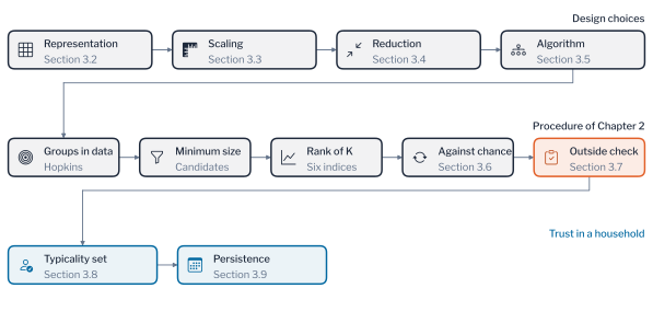
Figure 3.1 shows the order of the chapter. The choices of a design come first, the representation, the scaling and the reduction in turn, because every later stage works in the space that they define. The algorithm is treated with the number of groups, since the procedure of Chapter 2 selects the two together. Verification against chance and the outside check then test the selected design, and a last branch asks how far the group of a single household can be trusted.
Segmentation Task
A segmentation serves a decision such as a tariff offered to a class of customers or a demand-response programme aimed at a class [1]. It also serves a transformer study that represents many customers by a few profiles [2], [3], [4]. Utilities use such classes for network metrics [5]. The contribution of a customer to the coincident system peak can be estimated without a smart meter, from monthly bills and the typical daily patterns of metered customers [6], [7]. Low-voltage feeders are classified so that planning and hosting-capacity studies can represent many feeders by a few [8]. The two uses show what a class must preserve: the level of demand at the peak in the first, and the electrical characteristics of the feeder in the second. The decision fixes two inputs before any data are examined: the smallest group that the decision can use, and the evidence that must exist before the groups are acted on. The first enters the procedure as the minimum size of Chapter 2, nine households for a conformal threshold at a false-alarm rate of 0.1 and larger for a tariff offer. A tariff offer that needs 100 households in each group would allow at most 12 groups in London, 10 in GoiEner and 3 in AusNet. The second is an outside structure that no design has seen, the subject of Minority Groups.
A clustering design is the composition of the choices that turn the readings of a household into a label. With the representation \(\phi\) of Chapter 1 followed by a scaler \(\mathcal{T}\) and a reduction \(\mathcal{R}\), a design assigns household \(i\) the label
\[ \lambda(i) = \mathcal{M}_K\Bigl( \mathcal{R}\bigl( \mathcal{T} ( \phi(\mathbf{x}_i) ) \bigr) \Bigr), \tag{3.1}\]
where \(\mathcal{M}_K\) is the algorithm at \(K\) groups. Two designs that differ in any element partition the same households in different spaces. The silhouette of Equation 2.9 and the other internal indices are computed in the space of one design. They cannot rank designs that differ in \(\phi\), \(\mathcal{T}\) or \(\mathcal{R}\). Designs are compared instead by the agreement of their partitions, through Equation 2.2, which needs no shared space, and by the recovery of a structure established outside every design, through Equation 2.28. The comparison is made at one number of groups, the value that the procedure returns for a baseline design. The baseline is the seasonal profile of Chapter 1 without scaling, reduced by t-SNE and partitioned by k-means. Every comparison also shows the recovery over the whole range of \(K\), so that no conclusion rests on one value. The design that scores best then runs through the procedure again in Algorithms and Groups.
Three populations are used, because a finding that holds on one is a hypothesis about the others. Figure 3.2 shows them. The London population holds 1,284 households of the Low Carbon London trial, read every half hour. A dynamic time-of-use tariff was offered to part of the trial [9], and the tariff arm of each household is recorded. The GoiEner population holds 1,000 households of a Spanish cooperative, read every hour. They were drawn to stratify the residential status of the customers, and the cooperative’s records add the contract and activity fields. The AusNet population holds 342 households of a Victorian network, read every half hour for a year. The households are assigned to the network models of Chapters 4 to 6, and they carry no attribute at all. The utilities differ in country, climate, tariff and metering interval, so a result that holds on all three is unlikely to depend on the circumstances of one trial.
A segmentation of individual households also discloses behaviour. The half-hourly profile of one household shows when it is at home, so a representative profile built from few households reveals more about each of them. The minimum group size of Chapter 2 bounds the disclosure as well as the calibration. Each design is selected on the population and verified on a structure that is read only after the design is selected, so that selection and verification do not share information. This is the rule that separates model selection from assessment in supervised learning, applied to a task without labels [10]. Three practices follow from this rule in a utility. The decision fixes the minimum group size and the evidence before any data are examined. Every comparison reports the three populations together, so that no finding rests on one population. No design is selected on a structure that it is later verified against.
Remark: clustering has no held-out error
A supervised model is judged by its error on labelled data that it has not seen. A clustering has no labels, so its evidence is the separation of its groups, their reproducibility and their agreement with a structure outside the data [11], [12].
Representation of Households
A representation fixes what a distance can distinguish, and therefore what any clustering can find. A distance \(d\) is invariant to a transformation \(T\) of the readings when
\[ d\bigl(T(\mathbf{x}),\ T(\mathbf{y})\bigr) = d(\mathbf{x},\ \mathbf{y}), \tag{3.2}\]
and a clustering that uses \(d\) cannot separate households that differ only by \(T\). Two households with profiles \(\mathbf{x}\) and \(c\,\mathbf{x}\) for a constant \(c > 0\) are at the Euclidean distance \(\lvert c - 1 \rvert \, \lVert \mathbf{x} \rVert\) under the mean daily load. The peak-normalised shape \(\mathbf{s}\) of Equation 1.3 satisfies \(\mathbf{s}(c\,\mathbf{x}) = \mathbf{s}(\mathbf{x})\), so the same two households coincide. The representation is thus a statement about which differences are nuisance for the decision. Chapter 1 showed on the planted patterns that the normalised hour-of-day profile recovered timing exactly, while features of size and variability recovered none of it. That result states what carries timing; it does not state what matters on every metered population, and this section tests it on three.
Distances in a high-dimensional representation lose contrast, as Equation 1.12 states [13], [14], so a larger set is not better. A silhouette computed in a space of three columns cannot be compared with one computed in a space of 96. The Hopkins statistic of Equation 2.7 is computed for each representation, because Chapter 2 showed that a population can form groups in one space and a continuum in another.
Eleven representations are compared, the raw peak-normalised daily curve as the baseline and ten feature sets (Table 3.1). Three describe the year by season and by day of week and hour, and seven compress each household to a few summary statistics. For the daily consumption \(e_d\) of a household on day \(d\), with mean \(\bar{e}\) and standard deviation \(s_e\), the volatility set holds the coefficient of variation
\[ \mathrm{CV} = \frac{s_e}{\bar{e}}, \tag{3.3}\]
and the autocorrelation set holds the correlation of the daily series with itself at lag \(\ell\),
\[ r_\ell = \frac{\sum_{d} (e_d - \bar{e})(e_{d+\ell} - \bar{e})}{\sum_{d} (e_d - \bar{e})^2}. \tag{3.4}\]
| Set | Content | Dimension |
|---|---|---|
| Raw | Peak-normalised mean daily curve at hourly readings | 24 |
| Seasonal | Mean profile of each season by hour of day | 96 |
| Weekly | Mean profile of each day of the week by hour of day | 168 |
| Profile | Seasonal and weekly profiles together | 264 |
| Magnitude | Mean, spread and total of daily consumption | 5 |
| Volatility | Coefficient of variation and rolling spread | 2 |
| Trend | Recent day-on-day changes and the linear slope | 5 |
| Shape | Peak hour, morning-to-evening ratio and load factor | 3 |
| Autocorrelation | \(r_\ell\) at a few lags | 5 |
| Calendar | Weekday and weekend ratios and the peak-to-average ratio | 4 |
| Distribution | Skewness, kurtosis and quantiles of daily totals | 6 |
All eleven representations are specified in advance from the readings. A learned representation, such as the embedding of a deep clustering network [15], adapts to the data. It needs a large population and adds training choices that a utility must also validate. The simplest adequate representation is the one that preserves the structure of the decision.
Figure 3.3 reports the agreement between the partitions of the ten representations and the recovery of the outside structure of each population. The three profile representations agreed with the seasonal partition at an ARI of 0.53 to 0.88 on the three populations. The summary statistics were nearly unrelated to it, at no more than 0.10, and the raw daily curve agreed at 0.12 to 0.16. Size and volatility sort households by how much they consume and how erratic they are, and neither has a reason to reproduce a grouping by when electricity is used. The silhouette ranked the summary sets above the profiles, which reflects their dimension and not their quality. The three summary sets with the highest silhouette recovered 0.13 to 0.46 of the outside structure on London, and 0.18 to 0.32 on GoiEner. The three profile representations recovered 1.00 on London and 0.37 on GoiEner. The Spearman rank correlation of the two orders is \(\rho = 1 - 6 \sum_i \delta_i^2 / (n(n^2 - 1))\) for rank differences \(\delta_i\) of \(n\) sets. It was 0.12 on London and \(-0.15\) on GoiEner, so the order of the silhouette carries no information about the recovery. A representation is therefore not better or worse in the abstract. It determines which question the clustering answers, and where an outside structure exists, testing whether a representation preserves it is more informative than any index.
The raw curve compared with the seasonal profile also tests the distance. Dynamic time warping aligns two curves before comparing them. Chapter 1 found it worse than the Euclidean distance for shifts of up to one hour and better only at four hours. Warping also performs worse on the metered curves, where the Euclidean distance reached a silhouette of 0.15 on London and GoiEner and 0.23 on AusNet, against 0.08, 0.07 and 0.19. Household demand follows fixed times of day that are set by working hours, school timetables and tariff periods. A peak at seven and a peak at nine belong to different households and not to one household observed with a delay. A tariff or a demand-response event acts at a fixed hour, so a grouping that merges households whose peaks fall two hours apart merges households whose response differs.
Taken together, the comparisons show that the profile representations recovered the outside structure at 1.00 on London and 0.37 on GoiEner. The three summary sets with the highest silhouette recovered only 0.13 to 0.46 and 0.18 to 0.32. A utility that chose by silhouette would therefore segment customers by size and volatility and lose the timing of demand on which a tariff or a demand-response event acts. The peak-normalised profile with the Euclidean distance is the better choice, and any alternative should be tested against an outside structure.
Pitfall: choosing a representation without testing it
A representation with few columns has a high silhouette because distances in a low dimension separate more easily. Compare representations by their recovery of an outside structure, and use the silhouette only within one space. State the normalisation in the calling code as well, since a changed library default once turned every profile from when a household consumes into how much.
Scaling of Features
Let \(x_{ij}\) be feature \(j\) of household \(i\). Its mean is \(\mu_j\), its standard deviation \(\sigma_j\) and its median \(m_j\). Its interquartile range is \(q_j\), its minimum \(a_j\) and its maximum \(b_j\), and \(F_j\) is its empirical distribution function. Three scalers are affine maps of each feature. The standardised form subtracts the mean and divides by the standard deviation,
\[ t_{ij} = \frac{x_{ij} - \mu_j}{\sigma_j}. \tag{3.5}\]
The min-max form maps the range of the feature to the unit interval,
\[ t_{ij} = \frac{x_{ij} - a_j}{b_j - a_j}. \tag{3.6}\]
The robust form centres on the median and divides by the interquartile range,
\[ t_{ij} = \frac{x_{ij} - m_j}{q_j}. \tag{3.7}\]
The quantile transform replaces each value by its rank,
\[ t_{ij} = F_j(x_{ij}). \tag{3.8}\]
An affine scaler with scale \(s_j\) changes the squared Euclidean distance between households \(i\) and \(l\) to
\[ d^2(i, l) = \sum_{j=1}^{p} \frac{(x_{ij} - x_{lj})^2}{s_j^2}, \tag{3.9}\]
so each feature carries the weight \(s_j^{-2}\). Standardising sets \(s_j = \sigma_j\) and raises the weight of the hours in which households differ little, whereas peak-normalised hourly means already share a bounded scale. The power transform is the Yeo-Johnson family, a monotone map \(g_\lambda\). Its parameter \(\lambda_j\) is chosen for each feature by maximum likelihood, so that the transformed feature is as close to normal as possible [16]. The quantile transform of Equation 3.8 is monotone and not affine. In the tail of the distribution \(F_j\) is flat, so a large difference of two readings becomes a small difference of ranks. The transform compresses the tail in which a minority of households with extreme overnight demand lies. Standardising the variables changes how well clusters of known structure are recovered, and comparing methods of standardisation by that recovery is the test applied here to metered households [17].
Six conditions were compared on each population: no scaling, min-max, robust, standardising, the power transform and the quantile transform. The expectation from Equation 3.9 is that scaling adds nothing, because the weights of peak-normalised hourly means are already similar. Figure 3.4 shows the agreement of each partition with the unscaled one and the recovery of the outside structure. Across the six conditions the embedded silhouette varied by at most 0.06 and the balance stayed above 0.95. A choice made from a table of validity indices would treat the six as equivalent. Their partitions are nevertheless not equivalent, because standardising lowered the agreement with the unscaled partition to 0.64 on London and the quantile transform to 0.55 on AusNet. The indices do not measure what a scaler changes, and a practitioner who chooses a scaler from them is choosing among different segmentations of the customers without knowing it.
The unscaled partition scores 1.000 against itself by construction, so agreement cannot rank the conditions and recovery of the outside structure does. No scaling, min-max and robust scaling recovered it exactly on London, standardising 0.90 and the quantile transform 0.37. The order follows from the mechanism, because the quantile transform compresses the extreme overnight values that distinguish the minority group. Over ten seeds each condition was tested against no scaling by a Wilcoxon signed-rank test paired by seed. For each seed let \(\delta_s\) be the difference in recovery between a condition and no scaling, with \(R_s\) the rank of \(\lvert \delta_s \rvert\). The Wilcoxon signed-rank statistic is
\[ W = \sum_{s=1}^{10} \operatorname{sign}(\delta_s) \, R_s, \tag{3.10}\]
and under the hypothesis of no difference every sign pattern is equally likely, so that ten pairs of one sign have the two-sided probability \(2 / 2^{10} \approx 0.002\). Standardising, the power transform and the quantile transform were below no scaling in all ten seeds, which is the smallest probability that ten pairs allow. The ordering is a property of the conditions and not of the seed.
A scaler therefore changes which households are grouped together while leaving every validity index almost unchanged. No scaler improved on omitting the step, because the peak-normalised features already share a bounded scale, and three of the five made the recovery worse. Under the quantile transform only 0.37 of the 56 storage-heating households of London were recovered, against all of them without scaling. A storage-heating tariff would then reach about a third of its intended customers, and no index would signal the loss. The simplest adequate design therefore leaves the features unscaled and reports the recovery of an outside structure whenever a scaler is introduced.
A scaler is fitted on the households that fit the clustering and applied to new households with the same parameters. Refitting it on each batch changes the weights of Equation 3.9 without any change in behaviour. The conclusion is specific to this representation, and features in mixed units, such as kilometres of conductor, customers and kilovolt-amperes, reopen the question, which Further Applications returns to.
Dimension Reduction
The previous section left the peak-normalised features unscaled, so the households are still described by up to 96 columns. Distances between so many columns carry little contrast (Equation 1.12), and clustering algorithms are usually run on a reduced space. Reduction is the last design choice that acts on the features before the algorithm. Chapter 1 defined the reductions that this section compares: principal components, the kernel principal components of Equation 1.15, t-SNE (Equation 1.14), UMAP (Equation 1.16) and PaCMAP (Equation 1.17). It also defined the preservation \(P_k\) of Equation 1.18, the share of the \(k\) nearest households that survive a reduction. Chapter 2 supplied the connectivity of a neighbourhood graph and the balance of a partition. A reduction matters because the groups are found in the reduced space. One that scatters the neighbours of a household can split a group that exists in the readings. At \(k = 10\) the preservation of the metered households on London was 0.14 for principal components and for kernel principal components, 0.31 for t-SNE, 0.24 for UMAP and 0.19 for PaCMAP. The order was the same on GoiEner and AusNet, where t-SNE kept 0.34 and 0.37. The radial kernel at its default bandwidth behaved as the linear projection, so it is not a neighbourhood-preserving method here. The neighbourhood-preserving methods keep up to 2.2 times as many neighbours as the linear projection on London and 1.5 times on AusNet. None keeps more than 0.37, so every embedding remains a display and not a measurement. A utility should report the preservation and the smallest cluster beside the silhouette, run several seeds, and fit a reduction on the households that fit the clustering only. Six conditions are compared on each population: no reduction, principal components, kernel principal components with a radial kernel, t-SNE, UMAP and PaCMAP. Because each condition produces a different space, the silhouette is reported both within each embedding and in the shared feature space, where the partitions can be compared.
The two silhouettes disagree (Figure 3.5), since within each embedding reduction raised the silhouette, from 0.12 with no reduction on London to between 0.36 and 0.45 for the reduced embeddings. In the shared feature space the neighbourhood-preserving methods scored lowest, at 0.08 to 0.10 against 0.13 for principal components. The embedded silhouette rewards having fewer dimensions in which to separate, the effect that favoured the three-column summary sets. It cannot decide the question, whereas cluster sizes and balance can. At the number of groups of the baseline design the linear reductions returned a smallest cluster of 27 households on London, against 56 for the neighbourhood-preserving methods. The balance of the linear reductions was 0.88 and that of the neighbourhood-preserving methods 0.97. No separation index registers such a difference, because a small cluster far from the others is perfectly compact and perfectly separated. The balance of Equation 12.1 is the instrument of Chapter 2 that does.
The comparison is repeated on the other two populations in Figure 3.6 and Figure 3.7, because a result on London alone is a hypothesis about the others. On GoiEner no reduction recovered the non-residential customers well, with a recovery of 0.22 to 0.41. The smallest cluster held 24 to 37 households, so no reduction isolated a small group. The neighbourhood-preserving methods reached the highest recovery, at 0.38 to 0.41, and t-SNE and UMAP left the neighbourhood graph in three components. AusNet shows no separated structure under any reduction. Its two groups are the halves of a continuum, with a smallest cluster of 132 to 169 households. The reductions differ only in how cleanly they draw the boundary between the halves.
The connectivity check of Equation 2.8 explains part of the difference. Only t-SNE, UMAP and PaCMAP left the minority group of Minority Groups as a disconnected component of the ten-neighbour graph, and each isolated the same 56 households. Without reduction, and under principal components and kernel principal components, the graph had one component. The minority group is nevertheless not invisible without a neighbourhood-preserving method, since k-means recovered 0.96 of it on the unreduced features, but only those methods make it topologically distinct. Among them the choice matters little, because they agreed on the group exactly and their balance differed by 0.001. The neighbourhood-preserving methods are preferable, but their advantage on these populations is smaller than that of the representation. Chapter 1 warned that an embedding is a display and not a measurement, and the default settings of t-SNE do not suit every population [18]. The embedding is not read, but its neighbourhoods are the space in which the groups are found, so that choice has to be tested.
Each comparison above rests on one run of a stochastic reducer, so a difference could reflect the seed. The reducer and scaler comparisons were repeated over ten seeds on each population and each condition was tested against the baseline by a Wilcoxon signed-rank test paired by seed. The neighbourhood-preserving methods recovered the minority group exactly in every seed, with a smallest cluster equal to the group. The reduction by principal components recovered 0.91 of it in every seed, with a smallest cluster of 27 households (\(p = 0.002\) against t-SNE). K-means without reduction recovered 0.96 on average, with smallest clusters of 18 to 35 households. The two rules for the number of retained components disagree. The 90% variance rule asked for 11, 8 and 14 components on the three populations, and the profile-likelihood rule of Equation 1.19 asked for one. The disagreement matters little, because increasing the components retained by UMAP from two to twenty changed the balance on London by at most 0.004. The family of the reduction matters more than the number of components.
A reduction therefore cannot be judged by its silhouette, which rose for every reduction from 0.12 to between 0.36 and 0.45 on London. Only t-SNE, UMAP and PaCMAP isolated the 56 storage-heating households, whereas the linear reductions returned a smallest cluster of 27 and recovered 0.91 of the group. A utility should prefer a neighbourhood-preserving method and report its preservation and smallest cluster. A linear projection blurs the boundary of a minority of 56 customers, and a tariff aimed at them would be misdirected.
Algorithms and Groups
The design is now fixed up to the algorithm and \(K\), and the funnel of Chapter 2 applies from its first stage. On the chosen representation the Hopkins statistic of Equation 2.7 was 0.89 on London, 0.88 on GoiEner and 0.70 on AusNet. Uniform data of the same range gave 0.49 to 0.51. All three populations depart from a uniform spread, and AusNet departs least, as the 0.750 of its daily profile in Chapter 2 suggested. The structure of the planted patterns, 0.821, lies between the two groups of populations. The candidates are the values of \(K\) from 2 to 12, a wider range than the 2 to 8 of Chapter 2 because the populations hold 342 to 1,284 households. The minimum group size is nine households, the minimum of Chapter 2 for a conformal threshold at a false-alarm rate of 0.1. It removes no candidate on any population, because every partition into 12 groups or fewer has a smallest group above nine households.
Algorithms differ in what they take a cluster to be, so their agreement is informative only if their assumptions differ. The general reason is the impossibility theorem of Kleinberg [19], who studied which properties a clustering function can have. A clustering function \(f\) that maps a distance \(d\) to a partition satisfies scale invariance when \(f(\alpha d) = f(d)\) for every \(\alpha > 0\). It satisfies richness when every partition is the output for some \(d\), and consistency when shrinking the distances within groups and stretching those between groups leaves the partition unchanged. No clustering function satisfies the three together [19]. The choice of algorithm is therefore an assumption about the application and not a property of the data, and the comparison of this section is a comparison of assumptions.
Seven algorithms rest on the objective families of Chapter 1, and each optimises a different quantity. K-means and its mini-batch form minimise the within-group sum of squares of Equation 1.5. Ward linkage merges the two groups \(A\) and \(B\) whose union increases that sum least,
\[ \Delta(A, B) = \frac{\lvert A \rvert \, \lvert B \rvert}{\lvert A \rvert + \lvert B \rvert} \, \lVert \bar{\mathbf{x}}_A - \bar{\mathbf{x}}_B \rVert^2, \tag{3.11}\]
whereas average linkage merges the groups with the smallest mean pairwise distance,
\[ d(A, B) = \frac{1}{\lvert A \rvert \, \lvert B \rvert} \sum_{\mathbf{x} \in A} \sum_{\mathbf{y} \in B} d(\mathbf{x}, \mathbf{y}). \tag{3.12}\]
The Gaussian mixture maximises the likelihood of \(K\) components with weights \(\pi_k\),
\[ \ell = \sum_{i=1}^{N} \log \sum_{k=1}^{K} \pi_k \, \mathcal{N}(\mathbf{x}_i \mid \boldsymbol{\mu}_k, \boldsymbol{\Sigma}_k), \tag{3.13}\]
BIRCH summarises each subcluster of \(N\) households by the cluster feature
\[ \mathrm{CF} = \Bigl( N,\ \sum_{i} \mathbf{x}_i,\ \sum_{i} \lVert \mathbf{x}_i \rVert^2 \Bigr), \tag{3.14}\]
from which the centroid and the radius of the subcluster follow without the households, and it groups the summaries in a tree [20]. Spectral clustering minimises the normalised cut of Equation 1.8. A consensus of twenty k-means runs is added as an eighth. It forms the co-association matrix of Equation 2.13 from the twenty partitions and clusters \(\mathbf{1} - \mathbf{S}\). The principle is that the combination corrects the weakness of any one partition [21]. Each algorithm is ranked over the candidates by the weighted rank of Equation 2.20 with the six indices of Chapter 2 and the weights of Equation 2.19. Figure 3.8 shows the value of \(K\) that each algorithm recommends on each population and the adjusted Rand index between the partitions.
The algorithms divided according to what each of them assumes. On London six of the eight recommended two groups and spectral and average linkage recommended three. On GoiEner six recommended two, BIRCH five and spectral clustering eleven, and on AusNet five recommended two and Ward, BIRCH and average linkage three. Algorithms that partition on distance to a centre favour regions of similar size. Average linkage and spectral clustering respond to the largest gap in the data, so they can isolate a small group that the others divide. The coarsest division of a continuum has the highest separation, which is why the rank of most algorithms falls on two groups. The agreement of several algorithms is weaker evidence than it appears, because they share an objective and are ranked by the same indices on the same embedding. Agreement counts as evidence only when the algorithms differ in what they assume. A structure found by a partitioning, a density and a graph method alike does not depend on one definition of a cluster. The consensus of twenty runs returned the k-means partition with an adjusted Rand index of 0.99 on London. The agreement of the partitions in panels (b) to (d) shows the same division on each population. On London average linkage agreed with the other algorithms at 0.51 to 0.64, except with Ward at 0.85. On GoiEner spectral clustering and BIRCH agreed with the others at 0.15 to 0.32, whereas k-means, the mixture, Ward and mini-batch agreed at 0.69 to 0.99. On AusNet k-means, the mixture, mini-batch and the consensus agreed at 0.92 to 1.00. Ward, BIRCH and average linkage, which chose three groups, agreed with them at 0.35 to 0.46. The partitions diverge where the algorithms choose different numbers of groups, so the choice of an algorithm is a choice of \(K\) as much as of a method. On an embedding in which k-means is already stable across seeds, combining seeds has nothing to correct. The uncertainty of a household’s group is a property of the households and not of the algorithm.
In summary, most algorithms recommended two groups, six of eight on London and GoiEner and five on AusNet. On AusNet the excess of two groups was 0.023 against 0.154 for three. The agreement of algorithms that share an objective and an embedding is therefore not evidence of structure. A recommended number of groups is a proposal that the verification of the next section must test before a utility acts on it.
Figure 3.9 reconciles results that a reader of Chapter 2 would otherwise meet separately. On the AusNet households Chapter 2 clustered the peak-normalised daily profile without reduction, and every rule chose two groups, with a Hopkins statistic of 0.750. The seasonal profile after t-SNE, ranked by the same six indices, also recommends two groups. The two representations agree on the rank, but the mean excess of two groups is only 0.023. Three groups reach 0.154, the largest of any candidate. The verification of the next section keeps two groups as the highest-ranked candidate that passes, and the second rule of Chapter 2 selects three. A rank that is not verified is a proposal, and the weak excess of two groups shows that even a verified value can be marginal. The book uses the three groups of the second rule for the AusNet households in the chapters that place them on a network.
At the number of groups of the baseline design the groups of London hold between 56 and 224 households. Figure 3.10 places them in the embedding and shows their representative profiles with their sizes against the minimum, and the smallest group is the storage-heating group of Minority Groups. The profiles provide the check that no index performs. A high rank shows that the groups are separated, whereas only the curves show whether the separation corresponds to behaviour that a network planner would recognise. Figure 3.13 then summarises the stages of Chapter 2 on the three populations.
Figure 3.11 and Figure 3.12 show the baseline groups of the other two populations. On GoiEner the seven groups hold 37 to 197 households, and the smallest has almost no daytime demand and peaks at night. On AusNet the two groups hold 157 and 185 households. They peak at the same evening hours and differ in the amount of demand between midnight and the early afternoon.
Verification Against Chance
The fifth stage of the procedure asks whether the chosen number of groups reproduces better than structureless data. Chapter 2 defined the prediction strength, the stability of the least stable cluster and the subsample agreement. It showed that their chance level falls with \(K\), so that an uncalibrated check favours a coarse split by construction. The excess of Equation 2.17 and its mean of Equation 2.18 remove that dependence. The reference is data that are uniform over the range of each feature, as for the gap statistic [22]. A uniform reference is coarse for correlated features, because it fills regions that the households never occupy. A reference that permutes each feature keeps its distribution and breaks only the dependence between features. Either can be used when the check is repeated on five or more draws. The procedure takes the highest-ranked admissible candidate whose excess is positive on every check, which is the verified number of groups \(K_{\mathrm{v}}\) of Equation 2.27. The rule of Equation 2.26, which takes the largest mean excess in place of the highest rank, is reported beside it as a second rule.
Figure 3.14 shows the mean excess of the three checks on each population. On London the structureless reference reached a prediction strength of 0.95 at \(K = 2\) and 0.38 at \(K = 11\). The common threshold of 0.8 is therefore not one standard applied to different candidates, since noise exceeds it at small \(K\) and cannot exceed it at large \(K\). The rank chose two groups on all three populations, and the mean excess of two groups was \(-0.004\) on London, \(-0.019\) on GoiEner and 0.023 on AusNet. On London and GoiEner it is indistinguishable from the excess of a division of random points. The verification moved to seven groups on London and on GoiEner and kept two on AusNet, and the second rule chose seven, three and three. The two rules agreed on London and differed on the other two populations. The evidence is modest even where a check passes: on London none of the 11 candidates exceeded their reference by more than two standard deviations on all three checks. For an operator the consequence is that a high rank is not evidence of structure. The partition into seven groups on London is the best supported, and the partition into two groups that the indices prefer reproduces no better than noise.
The reference also qualifies what stability means, since the subsample agreement of Chapter 2 [23] never fell below 0.65 on structureless data. Two independent subsamples of uniform noise, clustered separately, agree substantially about which points belong together, because k-means partitions noise as reproducibly as it partitions anything. Stability therefore measures reproducibility and not structure, and the two coincide only where there is structure to reproduce. This is why the check is the excess and not the value. The confidence in the number of groups also differs by population. On London six of the eight algorithms recommended the same value, and on AusNet, the smallest population, five did, so the 342 households give the weakest basis for a consensus. A finding that holds on one population is a hypothesis about the others, and the size of the population limits the evidence that it can supply.
The rank preferred two groups on all three populations, with a mean excess of \(-0.004\) on London, \(-0.019\) on GoiEner and 0.023 on AusNet. The verification chose seven, seven and two groups, and the second rule seven, three and three. The reference reached a prediction strength of 0.95 at \(K = 2\), and its subsample agreement never fell below 0.65. A high rank or a high stability is therefore not evidence of groups. A two-class tariff on London or GoiEner would rest on a division that reproduces no better than noise. The utility should report the excess beside every chosen number of groups.
Remark: a ranked value is a proposal
The rank orders values of \(K\) by separation, and separation is high for any partition of a continuum into regions. Only a comparison with data that have no structure shows how much of a value’s reproducibility the population supplies. The procedure verifies the rank’s choice before using it.
Minority Groups
The sixth stage of the procedure compares the verified partition with a structure that no design has seen. Chapter 2 did so with an injected change on the synthetic population and showed two failures that a minority group provokes. The separation indices prefer an isolated cluster of few meters, and balance, which detects that failure, is itself lowered by a genuine minority. This section meets both failures on metered households. The outside structure is an attribute of the household where the records hold one and an injected change where they do not. It is read only after the design is selected.
Remark: an outside structure validates and does not label
An attribute such as a tariff arm or an activity code is evidence that the groups reflect behaviour. It is not the truth that the groups should reproduce, because households of one type behave in several ways, and an association is not a cause.
Storage Heating in London
The neighbourhood graph of the London embedding has two connected components, still two at fifty neighbours. The smaller joins the rest only at a hundred, so the structure is a gap between households and not a fragment of a particular neighbourhood. A graph with two components has two zero eigenvalues of its Laplacian (Equation 2.8), and a spectral method must separate the components before it can find anything finer [24]. The smaller component holds 56 households and coincides exactly with a spectral partition into two groups, at an ARI of 1.000. It is not an artefact of the embedding, since its silhouette was 0.414 in the 96-dimensional feature space against 0.369 in the plane.
Remark: off-peak storage heating
Storage heaters charge in a low-price night period and release heat through the day. A household that has them draws a large block of energy between midnight and the early morning. A dynamic time-of-use tariff changes the price by period, and a household on a legacy off-peak meter cannot take it.
The households form a recognisable behavioural group (Figure 3.15). Fifty of them reach their daily peak between midnight and one in the morning, against fewer than 1% of the others, whose median peak falls at seven in the evening. Sixty per cent of their daily consumption falls before six in the morning, against 15% for the rest, and their mean daily demand of 9.7 kWh is about double. A sharp overnight block and little consumption during the day is the signature of electric storage heating charged on an off-peak tariff. The tariff column of the trial confirms it independently (Figure 7.11). None of the 56 is in the dynamic time-of-use arm, against 18.6% of the rest of the population, which would have predicted about ten of them. Let \(n\) be the size of the group and \(m\) the number of the \(N\) households on the dynamic arm. Under independence of group and arm, the number \(X\) of group members on that arm has the hypergeometric distribution
\[ \Pr(X = x) = \frac{\binom{m}{x} \binom{N - m}{n - x}}{\binom{N}{n}}, \tag{3.15}\]
and Fisher’s exact test sums it over the tables at least as extreme as the observed one. It gives \(p \approx 2 \times 10^{-5}\). Their overnight peak is therefore not a response to the price signal of the trial, because none of them received it. It is pre-existing behaviour, consistent with a legacy off-peak meter on which a dynamic tariff cannot be layered.
The group is the metered instance of the failure that Chapter 2 demonstrated on planted data. It holds 4% of the population, so it exceeds the minimum size of nine and survives the filter. Its balance of 0.259 and its excess of zero at two groups both reject it, as they would reject a fabricated group. A balance gate removes a real minority exactly as it removes an artefact. A load that already runs overnight and is thermally buffered is a candidate for flexibility on the network, because its timing is already off the evening peak. A centroid method asked for the verified number of balanced regions cannot return a group that holds 4% of the households, so a segmentation built on it forfeits that group.
Detecting such a group requires an instrument that does not rank partitions. Connectivity does so, and so does a density method. DBSCAN calls a household a core point when its neighbourhood \(\mathcal{N}_\varepsilon(i) = \{ l : d(i, l) \leq \varepsilon \}\) holds at least \(m\) households, and a group is a maximal set of households joined through core points. The radius \(\varepsilon\) is read at the elbow of the sorted distances to the \(m\)-th neighbour [25]. The density-based validity index of a cluster \(C_i\) compares its density separation \(S_i\) from the other clusters with its density sparseness \(Q_i\),
\[ \mathrm{V}(C_i) = \frac{S_i - Q_i}{\max(S_i, Q_i)}, \qquad \mathrm{DBCV} = \sum_{i} \frac{\lvert C_i \rvert}{N} \, \mathrm{V}(C_i), \tag{3.16}\]
and is positive when the clusters are denser inside than between [26]. An inspection of the curves can also confirm a group.
The 56 households form a distinct group of 4% of the population, with 60% of their consumption before six in the morning and none on the dynamic arm. Balance and the excess rejected it, and only connectivity found it. A selection that relies on the rank alone would therefore discard a real group of off-peak load. Its timing is already off the evening peak, which makes it a candidate for flexibility, whereas it cannot take a dynamic tariff.
Pitfall: a balance gate removes a real minority
Balance and the calibrated excess both reject a genuine group of 4% of the households, as they reject an artefact. Check the connectivity of the neighbourhood graph before the rank, and read the groups that the rank rejects.
Customer Type in GoiEner
The GoiEner records give each household an economic activity code. The sample was stratified by residential status, so the code separates households (code 9820, 78.5% of the sample) from small businesses and other customers. A non-residential customer follows opening hours or a fixed schedule, so the groups of a design that preserves timing should separate the two types. The attribute is recorded and not injected, and the partition either reflects it or does not. The sample holds no night-rate contract, and only 10 households have registered photovoltaics, too few to support a statement.
Figure 3.17 shows, for each group of the baseline partition, the share of non-residential customers against its base rate of 21.5%, with Wilson intervals. For a group of \(n\) households of which a share \(\hat{p}\) is non-residential, the 95% Wilson interval is
\[ \frac{\hat{p} + z^2 / (2n) \pm z \sqrt{\hat{p}(1 - \hat{p})/n + z^2 / (4n^2)}}{1 + z^2 / n}, \qquad z = 1.96, \tag{3.17}\]
which stays within zero and one for the small groups of this chapter. Two groups concentrate the non-residential customers well above their base rate. Group 1 holds 159 households with the largest share of weekday daytime demand and is 64% non-residential. Group 3 holds 37 households with almost no weekday daytime demand and is 70% non-residential. The second group is consistent with loads that run at night, such as lighting, but the records do not state their purpose. The other five groups are between 3% and 18% non-residential. The partition agreed with the customer type at an ARI of 0.052. The permutation null repeats the comparison for \(B = 1000\) random permutations of the customer type, with the one-sided probability
\[ p = \frac{1 + \sum_{b=1}^{B} \mathbb{1}\left[ \mathrm{ARI}_b \geq \mathrm{ARI}_{\mathrm{obs}} \right]}{B + 1}, \tag{3.18}\]
and its distribution had a mean of 0.000 and a 95th percentile of 0.003, so no permutation reached the observed value and \(p < 0.001\).
The agreement is statistically clear but weak in size. Timing separates the non-residential customers whose schedule differs from that of a household, and it cannot separate those whose daily profile resembles one. The readings recover only a minority of the non-residential customers, so a tariff aimed at them cannot rely on the groups alone. An attribute that the demand does not reflect cannot validate a grouping, and the check reports honestly how far the demand reflects it.
Electric Vehicles in AusNet
The AusNet households carry no attribute, so the outside structure is an injected change. Forty households are chosen at random, 12, 15 and 13 from the three load patterns of the baseline design. A diversified Level-2 charging profile is added to every day of their year before the population is clustered again. The profile peaks at 1.49 kW per vehicle at 21:00 and is the diversified Level-2 profile of the book’s data. Its magnitude is physical and lies within the 0.3 to 12 kW range of a household peak. The experiment is semi-synthetic and the text, the caption and the scope remark say so. The structure is injected after the design is selected and read with the recovery, the cluster purity and the Jaccard overlap of Equation 2.28, Equation 2.29 and Equation 2.30.
The neighbourhood-preserving design isolated the adopters at every number of groups tested, from two to four, with a recall, a purity and a Jaccard overlap of 1.00 (Figure 10.4). The linear design isolated them only from three groups: at two groups the adopters shared a group with 96 other households, so the purity fell to 0.55. The adopters are seen because the evening charging of 1.49 kW moves a household’s normalised profile far from the others. The change also reorganised the rest of the population. The agreement of the other households with their partition before the injection, measured by the adjusted Rand index, was 0.00 at two groups, 0.51 at three and 0.62 at four. A group of adopters therefore displaces a group of the existing partition and moves other households with it. A monitoring schedule should compare the partitions of successive periods and should not look only for a new group. The design that preserves timing is the more sensitive, because the linear reduction needs one group more to separate the adopters.
The design that preserves neighbourhoods isolated all forty adopters at two, three and four groups, with a recall, purity and overlap of 1.00. The linear design needed three groups, and at two the purity fell to 0.55. The injection also moved other households, whose agreement with their earlier partition was 0.00 at two groups. A monitoring programme that looks only for a new group would therefore misread the change. It should use a design that preserves timing and compare the partitions of successive periods.
Missing Readings
The design was selected on complete records, and a distribution operator rarely holds them. Smart meters lose readings to communication failures, and some collection systems report at two or four times the interval of the trial. Two degradations test whether the design and its outside check survive. A random share of the readings is removed before the seasonal profile is computed, which is data that are missing completely at random in the sense of Rubin [27]. The readings are also averaged to a two-hour interval. The profile is the mean of the available readings at each hour of the day. A missing reading therefore shortens the sample of an hour and does not set it to zero.
Each condition repeats the baseline design at the baseline number of groups and is compared in Figure 3.19 with the baseline partition and with the outside structure. A change of the t-SNE seed serves as the reference. It reproduced the baseline partition on all three populations, at an adjusted Rand index of 1.00. Any lower agreement is therefore an effect of the degradation and not of the seed.
On London, removing 10% and 20% of the readings lowered the agreement with the baseline partition to 0.70, yet all 56 storage-heating households were still recovered. At 40% the agreement was 0.55 and the recovery 0.95. The two-hour interval did more damage than the missing readings. The agreement fell to 0.31 and the recovery to 0.69, so about a third of the storage-heating households were no longer found. The outside structure of GoiEner was recovered at 0.36 to 0.39 in every condition, as at the baseline, because the profile represents it weakly. On AusNet the agreement was 0.66, 0.84 and 0.75 for the three shares of missing readings and 0.33 for the two-hour interval.
Missing readings changed the assignment of many households, to an agreement of 0.55 to 0.84 with the baseline. The minority group of London survived 20% and was still 95% recovered at 40%. A two-hour interval reduced the agreement to 0.31 to 0.48 on every population and the recovery on London to 0.69. An operator whose meters lose a fifth of their readings can therefore still find a distinct minority group. Many assignments change, so the share of missing readings should be reported beside the groups. Two-hour readings cannot support the design for a minority such as storage heating, because the overnight block that identifies it is averaged into the neighbouring hours.
Certainty of Membership
A partition assigns every household to one group, including households that lie near a boundary and households that lie far from every representative profile. A decision that acts on the group, a class tariff for example, needs to know which assignments it can rely on. The assignment is therefore replaced by a prediction set, a map \(\Gamma\) from a household to a subset of the \(K\) groups. The size of the set reports how well the partition describes the household. Conformal prediction builds such a set from a nonconformity score, which is large when a household is atypical of the groups. It also needs a calibration set of households that the clusterer has not seen [28], [29]. Its split form needs no density model and no retraining [30], [31]. The clusterer is fitted on a random 70% of the households and the representative profile \(\mathbf{c}_k\) of each group is kept. A further 15% calibrate a threshold, and the last 15% are left to test the sets. For a calibration household \(i\) the nonconformity score is the distance to its nearest representative profile, \(r_i = \min_k d(\phi_i, \mathbf{c}_k)\). It is computed in the feature space, so that it has the units of the peak-normalised profile and not of an embedding. For \(n\) calibration households and a miscoverage level \(\alpha\), the threshold \(\hat q\) is the \(\lceil (n + 1)(1 - \alpha) \rceil\)-th smallest score, and every household receives the set
\[ \Gamma(i) = \{\, k : d(\phi_i, \mathbf{c}_k) \le \hat q \,\}. \tag{3.19}\]
Three conditions give the guarantee: the representative profiles are fixed before the calibration households are scored, the calibration and test households are exchangeable, and the threshold is the quantile above. Exchangeability makes the rank of the score \(r_{n+1}\) of a new household uniform on \(\{1, \dots, n + 1\}\). The probability \(\Pr(r_{n+1} \le \hat q)\) is then the share of ranks not above \(\lceil (n + 1)(1 - \alpha) \rceil\). The share is at least \(1 - \alpha\), and it exceeds \(1 - \alpha\) by less than \(1/(n + 1)\) when the scores have no ties:
\[ 1 - \alpha \le \Pr\bigl( r_{n+1} \le \hat{q} \bigr) \le 1 - \alpha + \frac{1}{n + 1}. \tag{3.20}\]
The nearest representative profile of a new household therefore lies within \(\hat q\) with at least that probability, and its set is not empty with that probability. The quantile exists only when \(\lceil (n + 1)(1 - \alpha) \rceil \le n\), that is, when \(n \ge (1 - \alpha)/\alpha\). At \(\alpha = 0.1\) this gives the nine households of the minimum group size above. The coverage is marginal over households and not conditional on the group, which needs further conditions [32]. A threshold calibrated within each group would give coverage for each group, at the price of a larger calibration set for every group. The guarantee concerns typicality and not the true group, because no true group exists. It is the construction used to test for outliers with conformal p-values [33]. The nearest-distance score could be replaced by a margin, the distance to the second-nearest profile minus that to the nearest. A margin separates boundary households from others but cannot flag a household that is far from every group. A set of one group is a confident assignment, and a set of two marks a household on a boundary. An empty set marks a household that no group describes as well as the calibration households were described.
The set is compared with the soft assignment of a Gaussian mixture. The mixture gives household \(i\) the posterior probability of group \(k\),
\[ \gamma_{ik} = \frac{\pi_k \, \mathcal{N}(\mathbf{x}_i \mid \boldsymbol{\mu}_k, \boldsymbol{\Sigma}_k)}{\sum_{l=1}^{K} \pi_l \, \mathcal{N}(\mathbf{x}_i \mid \boldsymbol{\mu}_l, \boldsymbol{\Sigma}_l)}, \tag{3.21}\]
and reports the groups with \(\gamma_{ik} \geq 0.1\). The two sets answer different questions about the same household. The mixture states how the model divides probability among groups, and its probabilities are only as calibrated as its density model. The conformal set states how typical a household is of the groups, and its coverage holds without a density model. Figure 5.14 reports both on the test households, never on those that fitted the clusterer or calibrated the threshold, over ten random splits and for two to seven groups.
At seven groups on London 14.5% of the test households received one group, 76.1% received two or more and 9.4% received none. The empty share stayed within the \(\alpha = 0.1\) that the construction allows. The shares on GoiEner were 13.8%, 77.9% and 8.3%, and on AusNet at five groups 11% received one group. The share of single-group households fell from 37% at two groups to 15% at three on London and stayed there. The groups divide a continuum, so most households lie within the calibrated radius of the representative profiles of several groups. The mixture reported more than one group for only 5% of the London households. Its posteriors in 96 dimensions are far more confident than the geometry of the households supports. A programme that acts on a group should therefore treat a household with an uncertain set as unassigned. It cannot read the confidence of a mixture as a measure of certainty.
Pitfall: reading a typicality set as a probability
A set of two groups does not say that the household belongs to each with probability one half. It says that the household lies within the calibrated radius of both profiles. Use the set to decide whether to act on a label, and not to weight a decision.
The guarantee depends on exchangeability, so it was tested on households of a different period. The threshold was calibrated on the households of the first quarter, and the sets were assigned to the households of the last quarter. The share of non-empty sets was 0.90 on London, 0.89 on GoiEner and 0.83 on AusNet, against 0.89, 0.89 and 0.88 within the first quarter. The coverage held where the households keep their position relative to their representative profiles and fell on the population with the least stable groups. Conformal methods that relax exchangeability or correct for covariate shift address such departures [34], [35]. A utility should recalibrate on the period in which it acts.
At seven groups on London 14.5% of the test households received one group, 76.1% two or more and 9.4% none, and the mixture reported more than one group for 5%. In a later quarter the share of non-empty sets was 0.90, 0.89 and 0.83. Most households therefore cannot be assigned to a single group with confidence. A programme should treat a household with an uncertain set as unassigned and recalibrate the threshold for the period in which it acts.
Persistence and History
A group can inform a persistent decision, a tariff or a connection approval, only if a household keeps it. The daily load shape of one household varies considerably from day to day [36], so persistence cannot be assumed. Each quarter is clustered separately with the design of the previous sections. The labels of two partitions are arbitrary, so the groups of one quarter are matched to those of the next before households are compared. Matching is an assignment problem solved by the Hungarian method [37]. Among the permutations \(\pi\) of the \(K\) groups, the matched partition maximises the number of households that keep their group,
\[ \pi^{*} = \arg\max_{\pi} \sum_{k=1}^{K} \bigl\lvert C^{(1)}_{k} \cap C^{(2)}_{\pi(k)} \bigr\rvert, \tag{3.22}\]
and the share of households that changed group between the two quarters is
\[ \tau = 1 - \frac{1}{N} \sum_{k=1}^{K} \bigl\lvert C^{(1)}_{k} \cap C^{(2)}_{\pi^{*}(k)} \bigr\rvert. \tag{3.23}\]
The matching is the most favourable reading, since it counts every household that could have kept its group as having kept it. The turnover it reports is a lower bound. Households that change group may do so because their behaviour changed or because the partition of a continuum places a boundary differently when the data move slightly. The two causes are separated by a baseline. Each household’s days are resampled within its own year to form two pseudo-periods. The agreement of their partitions is what would be expected if each household behaved exactly as in its own year.
Figure 3.21 reports the matched transitions between the first and last quarters on the three populations and the agreement of consecutive quarters against that baseline. Partitions of consecutive quarters agreed at an ARI of 0.23 on London, 0.18 on GoiEner and 0.29 on AusNet. The baseline in which each household behaves as in its own year agreed at 0.31, 0.31 and 0.43. Partitions of the same quarter with other seeds agreed at 0.69, 0.73 and 1.00. Consecutive quarters agree less than the baseline does, so the change between quarters is more than the sampling of days. It combines the seasonal change of demand with the change in the behaviour of households. It is not an effect of the algorithm, because the same quarter clustered again reproduces much better. Under the matching, 50% of the London households changed group between the first and the last quarter. The share was 63% on GoiEner, with seven groups, and 29% on AusNet, with two. A label stored from one quarter was therefore wrong for half of the households by the end of the year, and nothing in the stored label indicates which. Groups that inform persistent decisions must be recomputed on a schedule, and the turnover between runs is itself a quantity to monitor.
The same sensitivity to behaviour makes the groups an instrument for monitoring, which the injected change of Minority Groups showed, and both uses depend on how much record is clustered. For a window of \(w\) days, the agreement with the partition of the whole record is the adjusted Rand index of the two on the households that they share,
\[ a(w) = \mathrm{ARI}\bigl( \lambda_{w},\ \lambda_{\text{record}} \bigr), \tag{3.24}\]
and its growth with \(w\) is a learning curve of the partition. Figure 3.22 clusters the mean daily shape of the first day, week, month and season. On London a single day agreed with the record at 0.05, a week at 0.14, a month at 0.28 and a season at 0.31. The curves of GoiEner and AusNet are lower for short windows, and AusNet reaches 0.29 only at a season while GoiEner stays near 0.16 from a month. A week can be as well separated as a day while agreeing with the record several times as closely. The silhouette of a short window says little about the households it describes. A newly metered household can be assigned to a group only provisionally, and even a season of readings reproduces about a third of the partition of the year. A programme that segments customers at connection must use the typicality sets of the previous section, which state the uncertainty of an early assignment, instead of a single label. A re-clustering detects a change of behaviour only once the changed behaviour fills most of the window.
Consecutive quarters agreed at an ARI of 0.23, 0.18 and 0.29, below the baselines of 0.31, 0.31 and 0.43, and 50% of the London households changed group within the year. A season of readings reproduced 0.31 of the partition of the year. A stored label was therefore wrong for about half of the households by the end of the year. Groups must be recomputed on a schedule, and a newly metered household receives a provisional assignment only.
Pitfall: storing a group as a customer attribute
A group computed from one period describes that period. A label stored as an attribute of the customer ages without any sign in the record, so recompute it on a schedule and track the turnover between runs.
Further Applications
The procedure of this chapter applies to any clustering whose result informs a decision on the low-voltage network. It compares a design through the agreement of partitions and an outside structure, and then verifies it against chance. Four problems of the low-voltage network use it directly.
The first is the assignment of a tariff by class. A household offered a tariff designed for its group receives the wrong one if it changes group within the year. A utility can restrict class-based offers to the households whose typicality set holds a single group in every quarter and treat the others individually. The trial’s own tariff arm supplies the check. A segmentation that does not separate the households that responded to a price from those that did not has little value for tariff design, whatever its indices. The second is the detection of a new technology behind the meter. The injected change of Minority Groups added charging to forty households and found them as a group of their own. The same comparison of consecutive quarters flags households that leave their group together, which is the signature of a new vehicle, heat pump or battery. Methods that disaggregate behind-the-meter generation from net demand estimate the same quantity from a different direction [38], [39].
The third is the selection of a sample of households for a trial or a survey. A sample stratified by group represents the shapes of demand of the population. The typicality sets state which households represent their group well, so a trial drawn from the confident members of each group tests the groups and not their boundaries. The fourth is the selection of representative feeders for network studies. A distribution operator cannot model every feeder in detail and studies a few representatives of groups of feeders, chosen by clustering their length, customers and loading [8], [40]. These features are in different units, which is the case that the scaling comparison of this chapter warned would reopen the question. The feeder representatives must therefore be verified with the same comparison of scalers before they stand for the network.
Decision Table
A utility applies the chapter in the following order.
- State the decision, its minimum group size and the evidence that must exist before the groups are acted on (Segmentation Task).
- Specify a representation that keeps what the decision needs, test whether the population has groups in it, and prefer the simplest adequate set (Representation of Households).
- Leave peak-normalised features unscaled unless a comparison on an outside structure shows a gain, and prefer a neighbourhood-preserving reduction that reports its preservation and its smallest group.
- Rank the candidate numbers of groups for several algorithms with the six indices, remove those below the minimum size, and verify the selected value against structureless data (Algorithms and Groups).
- Read the outside structure after the design is selected, and run the connectivity check beside the rank so that a minority group is not removed (Minority Groups).
- State a typicality set for each household and a schedule on which the groups are recomputed.
Table 3.2 sets out how the choices of this chapter depend on what the utility has. It extends the guides of Chapters 1 and 2, which choose a method and a validation by purpose, with the context of the data.
| Context | Representation | Scaling and reduction | Number of groups | Verification |
|---|---|---|---|---|
| An outside attribute is recorded (a tariff, a contract) | Peak-normalised profile, seasonal | None; neighbourhood-preserving reduction | Procedure of Chapter 2 | Association with the attribute and a permutation null |
| No attribute; a change can be injected | Peak-normalised profile, seasonal | None; neighbourhood-preserving reduction | Procedure of Chapter 2 | Recovery of the injected change |
| Fewer than about 500 households | Peak-normalised profile | None; linear reduction only if sizes stay above the minimum | Rank verified against chance, with a wide margin | Calibrated excess; expect a weak consensus |
| Meters that lose readings or report every two hours | Peak-normalised profile from the mean of available readings | None; neighbourhood-preserving reduction | Procedure of Chapter 2 | Report the share missing; a minority group needs a half-hourly or hourly interval |
| Hourly interval | Seasonal profile of 24 hours | None | As above | As above |
| Newly metered customers | Mean daily shape of the first season | None | Typicality sets, not a single label | Recompute on a schedule; track turnover |
Conclusion
This chapter asked two questions of three metered populations. The first was whether the design that recovered the planted patterns of Chapter 2 still serves when no structure is known, and how its choices are verified without labels. The design survived: the peak-normalised seasonal profile, unscaled and reduced by a neighbourhood-preserving method, preserved the outside structure that the indices could not see. The representation mattered more than any other choice, and the quantile transform was the only scaler that dissolved the minority group on London. The rank proposed a number of groups and the verification against chance decided it, so a proposal and a verified answer were never confused. A minority group that every ranking criterion rejected, the storage-heating households of London, was found by connectivity and confirmed by the trial’s tariff. The customer type in GoiEner and an injected change in AusNet tested the same procedure.
Key findings
The unscaled seasonal profile, reduced by a neighbourhood-preserving method, preserved the outside structure of London and more weakly that of GoiEner. The representations and scalers that dissolved it scored as well on the indices. The rank proposed a number of groups and only the comparison with structureless data verified it. A minority group rejected by every ranking criterion was found by connectivity. A household’s group should be recomputed each season and treated as unassigned when its typicality set is uncertain.
The second question was how far the group assigned to one household can be trusted, and the answer is that it can be trusted less than its separation suggests. Half of the London households changed group within a year, and most lay within the radius of more than one group or of none. Even a season of readings reproduced only about a third of the partition of the year. A group is therefore a property of a period and not of a household. It is useful for monitoring change and unsafe as a stored attribute, and a utility that acts on it should recompute it on a schedule.
Remark: scope and limitations
Each population has one independent structure, and no result concerns the outcome of a decision. The households are metered but not located, so geographical clustering of behaviour is outside the evidence. An automated search over the design optimises the indices that this chapter shows to be misleading, so it inherits their limits and is not a substitute for the outside check.
The results describe the groups on their own terms and do not show whether they bear on the risks that motivate their use. Chapter 4 places the same households on a real network and asks whether the groups predict where violations of voltage and loading occur.
Exercises
- Show that the Laplacian \(\mathbf{L} = \mathbf{D} - \mathbf{W}\) of an undirected graph with \(c\) connected components has the eigenvalue zero with multiplicity \(c\). Conclude that a spectral partition into \(K < c\) groups cannot separate the components.
- Under random assignment of \(N\) points to \(K\) groups of equal size, show that two points share a group with probability \(1/K\). Explain why the prediction strength of Equation 2.14, a minimum over the clusters of a quantity with this chance level, falls faster with \(K\) than the chance level itself.
- A utility holds the hourly profiles of 60,000 households, no topology records and no attribute, and wants three groups for a tariff offer. Choose the representation, the reduction, the verification and the minimum group size, and justify each from Table 3.2 and Chapter 2. State which choice changes if the groups must inform the sizing of transformers.
- In the
connectivitycell of the companion notebook, compute the components of the neighbourhood graph on the GoiEner and AusNet embeddings. Does either population contain a disconnected group, and if so, what does its mean daily profile show? - Repeat the scaler comparison of the
scalerscell with the weekly profile in place of the seasonal profile. Does the ordering of the scalers by recovery persist? - Run a multi-objective search over the representation, the scaler, the reduction, the algorithm and \(K\) on one population, with the density silhouette, the balance and a resampling proxy as objectives. Compare the non-dominated trials with the outside structure of the population. Do any recover it better than the design of this chapter?
- Change the miscoverage level \(\alpha\) of the
setscell from 0.1 to 0.2 and to 0.05. How do the shares of empty sets and of sets of two follow \(\alpha\), and why does the share of sets of one group not follow it?