Foundations of Anomaly Detection
The analyses of Parts 5 and 6 assume that the readings of every meter are correct and that the behaviour of every customer is stable. In the operation of a distribution network, neither assumption holds without verification. A frozen register reports one value for several hours, a communication fault replaces readings with zeros, a meter out of calibration reports a constant multiple of the true demand, and a tampered meter under-records it. An inverter may export at an unusual hour, and the purchase of an Electric Vehicle (EV) changes a household’s evening demand permanently. Undetected, each of these conditions enters the clusters of Part 5 and the case base of Part 6, and each must be distinguished from the ordinary variation of a household’s demand between days.
Anomaly detection is the statistical problem of identifying observations that do not conform to the behaviour that generated the remainder of the data [1]. It differs from the classification of faults in that labelled anomalies are rare or absent. A detector is therefore fitted to normal data only, and it assigns each new observation a score that measures its departure from the normal data. Three questions have to be settled before such a detector is applied to a network. The first is which representation of a day and which family of detectors suit which kind of anomaly, since a representation determines the departures that remain visible and each family of detectors adopts a different definition of departure. The second is how a score is converted into a decision whose rate of false alarms is known before deployment. The third is how a detector is evaluated in the absence of labelled anomalies.
This chapter reviews the literature on the three questions, states the problem in the notation of the book, and examines each question on a synthetic metered population into which faults of known kind are injected, so that the presence of every anomaly is known. It also treats two topics that follow the raising of an alarm: the identification of the readings responsible for a flag, and the distinction between an anomaly and a change of normal behaviour. Chapter 2 applies these methods to the customers of the AusNet network, and Chapter 3 to the violations of its transformers.
Each section teaches a machine-learning concept on an LV problem and sets it against alternatives resting on other assumptions.
Anomaly Detection in the Literature
The review follows the three questions in turn: the kinds of anomaly and the detectors suited to them, the conversion of scores into decisions, and the evaluation of detectors. It closes with the applications to smart-meter data.
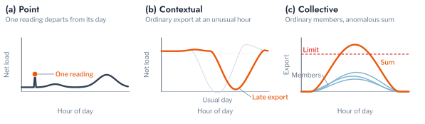
Chandola, Banerjee and Kumar distinguished three kinds of anomaly. A point anomaly is an observation that is anomalous on its own, a contextual anomaly is anomalous only with respect to a context such as the time of day, and a collective anomaly is a group of observations that is anomalous as a whole although each member may be ordinary [1]. Aggarwal’s monograph classifies detectors by the definition of departure on which they rest [2]. Distance-based detectors score an observation by its distance to its nearest neighbours [3]. Density-based detectors score it by the density of its neighbourhood relative to that of its neighbours [4] or by a kernel estimate of the density [5], and boundary methods by its position relative to a surface that encloses the normal data [6], [7]. The Isolation Forest scores an observation by the number of random splits required to isolate it [8], and Empirical-Cumulative-Distribution-Based Outlier Detection (ECOD) and Copula-Based Outlier Detection (COPOD) by the tail probabilities of each of its features under the empirical distribution [9], [10]. Robust estimates of location and covariance yield the Mahalanobis distance [11], and the Shewhart control chart, the earliest of these methods, flags a reading that lies more than three standard deviations from its mean [12]. Murphy presents the probabilistic basis of these methods, from the Mahalanobis distance and kernel density estimation to the detection of out-of-distribution inputs [13], [14].
No detector is superior on every dataset. Comparisons of tens of detectors on tens of datasets found that their ranking varies between datasets and that simple detectors frequently equal complex ones [15], [16], [17]. Ruff and colleagues unified shallow and deep detectors within one framework, and Pang and colleagues reviewed deep detectors, whose advantage is greatest on images and text rather than on short tabular records such as a day of readings [18], [19]. A combination of detectors reduces the dependence on any single one, and Aggarwal and Sathe analysed such ensembles in terms of bias and variance [20], [21].
The input of a detector is itself a choice. In many dimensions, distances between observations concentrate, and a detector applied to every reading of a series becomes sensitive to irrelevant variation [22]. Feature-based analysis of time series therefore represents a series by a small number of interpretable features, a practice that Fulcher and Jones applied to classification [23], Christ and colleagues automated by hypothesis tests on each feature [24], and Hyndman and colleagues and Talagala and colleagues applied to the detection of anomalous series [25], [26]. Events are a feature-based representation with a physical basis. The theory of extreme values treats the exceedances of a threshold and their runs as the object of analysis [27], and power-quality practice characterises a voltage disturbance by its depth and duration [28]. Part 5 described the violations of a transformer by the duration, depth and timing of their events (Equation 4.17), with the time of day encoded on the unit circle [29], and Part 6 ranked transformers by the summed severity of their events (Equation 8.1).
A score requires a threshold before it yields a decision. The threshold is commonly a percentile of the training scores, and its rate of false alarms on new data is then unknown. Conformal anomaly detection calibrates the threshold on held-out normal data instead, which bounds the probability of flagging a new normal observation [30], [31], [32]. Bates and colleagues formulated the same test with conformal p-values and showed that these permit control of the false discovery rate when many observations are tested simultaneously [33], [34], and Marandon and colleagues extended this control to detectors adapted to the data [35]. A change of normal behaviour, as distinct from the departure of a single observation, is the subject of change-point detection, from the cumulative sum of Page to the exact segmentation of Killick and colleagues [36], [37], [38], [39], and of the literature on concept drift in machine learning [40]. Shapley values attribute a score to the features of an observation and so provide an explanation of a flag [41], [42].
The evaluation of detectors presents difficulties of its own. Kim and colleagues showed that point adjustment, a common protocol for time series that counts an anomalous segment as detected in full when one of its points is flagged, permits a random score to equal the reported performance of published detectors [43]. Wu and Keogh, and Liu and Paparrizos, found that widely used benchmarks contain trivial or mislabelled anomalies [44], [45].
For smart-meter data, the reviews of Wang and colleagues and of Himeur and colleagues include anomaly detection among the principal analytics of metered consumption [46], [47], and Moghaddass and Wang organised detection hierarchically, from the meter to the transformer [48]. Non-technical loss, the energy consumed but not recorded, has been reviewed by Messinis and Hatziargyriou and by Glauner and colleagues, who identify the scarcity of labelled cases as the principal limitation of its detection [49], [50]. Faults of PV systems have been reviewed by Mellit, Tina and Kalogirou [51], and Patrizi and colleagues reported that a three-sigma control limit was competitive with more complex detectors for the power quality measured by smart meters [52]. Wang and colleagues reviewed the causes of alarm overload in industrial operation, to which a detector with an uncontrolled rate of false alarms contributes [53]. These studies address individual steps, and few evaluate a detector against anomalies whose presence is known. The following section states the problem in a form that admits such an evaluation.
Problem Formulation and Notation
The readings of meter \(i\) on day \(d\) form a vector \(\mathbf{x}_{i,d} \in \mathbb{R}^{T}\), with \(T = 48\) half-hourly readings of net load and export taken as negative. A detector is fitted on a set \(\mathcal{D}^{\mathrm{tr}}\) of days assumed to be normal and assigns to every day an anomaly score \(s(\mathbf{x})\), which increases with the departure of the day from the training days. A threshold \(\tau\) converts the score into a decision, and a day is flagged when
\[ s(\mathbf{x}_{i,d}) > \tau. \tag{10.1}\]
Two error rates characterise the decision. The false-alarm rate is the probability of flagging a normal day, and the recall is the probability of flagging an anomalous day.
In statistical terms, detection is a test of the hypothesis that a day was drawn from the distribution \(P_0\) of normal days,
\[ H_0 : \mathbf{x} \sim P_0, \tag{10.2}\]
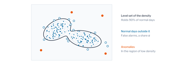
against the alternative that it was not. The false-alarm rate is the probability of a type I error, the rejection of \(H_0\) for a normal day, and the recall is the power of the test. When the distribution \(P_1\) of anomalous days is known, the lemma of Neyman and Pearson shows that the most powerful test at a given false-alarm rate is a threshold on the likelihood ratio \(p_1(\mathbf{x}) / p_0(\mathbf{x})\) of the two densities [54]. The distribution of anomalies is not known in practice. If no form of anomaly is preferred, so that \(p_1\) is taken as uniform over the range of the readings, the test becomes a threshold on the density of normal days alone, and the days that are not flagged form a level set of that density,
\[ \mathcal{L}_\lambda = \{ \mathbf{x} : p_0(\mathbf{x}) \ge \lambda \}, \tag{10.3}\]
with the level \(\lambda\) chosen so that the set holds a share \(1 - \alpha\) of the normal days. Among all sets that hold this share, the level set has the smallest volume, and its estimation from normal days is the formal statement of anomaly detection [55], [56]. Each detector of this chapter replaces \(p_0\) with a score that orders the days approximately as the density does (Figure 10.1). The level set also formalises the definition of Hawkins, for whom an outlier is an observation that deviates so much from the others as to suggest that it was generated by a different mechanism [57].
The three kinds of anomaly of Figure 10.3 take a precise form in these terms. A point anomaly is a day of low density \(p_0(\mathbf{x})\). A contextual anomaly is a day that is ordinary under the marginal density but improbable given its context \(\mathbf{c}\), such as the hour of an export or the weather, so that its conditional density \(p_0(\mathbf{x} \mid \mathbf{c})\) is low. A collective anomaly is a set of observations, such as the days of the customers of one transformer, whose joint density is low although the density of each member is ordinary. The setting of this chapter is that of novelty detection, in which the detector is fitted on days assumed to be normal and no labels are used. Unsupervised detection fits on data that may contain anomalies, and supervised detection requires labelled anomalies, which in metering are rare and of uncertain completeness [50].
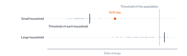
A detector fitted on the days of one household is a self-baseline detector. It compares the household with its own history rather than with the population, so that a household with a high level of demand is not flagged on account of its level (Figure 10.2). Figure 10.3 illustrates the kinds of anomaly to be detected, and Table 10.1 collects the notation, which extends that of Parts 5 and 6 (Table 1.1, Table 6.2).
Pitfall: anomalies among the training days
A detector fitted on days assumed to be normal learns any faults that those days contain, and assigns low scores to recurrences of them. Robust estimates of location and spread, such as the minimum covariance determinant and the median, limit the influence of a minority of faulty days, and the contamination share of most libraries assumes a known proportion of them. The protocol of this chapter injects faults only into held-out days, so that the training days are normal by construction; measured days, as in Chapter 2, offer no such guarantee.
| Symbol | Description |
|---|---|
| \(\mathbf{x}_{i,d}\), \(T\) | Readings of meter \(i\) on day \(d\), and readings per day |
| \(s(\mathbf{x})\), \(\tau\) | Anomaly score and threshold |
| \(\mathcal{D}^{\mathrm{tr}}\), \(\mathcal{D}^{\mathrm{cal}}\) | Training days and \(n\) calibration days, both normal |
| \(\alpha\) | Target false-alarm rate, or target false discovery rate |
| \(P_0\), \(p_0\), \(\mathcal{L}_\lambda\) | Distribution and density of normal days, and their level set at level \(\lambda\) |
| \(\pi\) | Share of anomalous days, the prevalence |
| \(\Phi^{-1}\), \(s^{\ast}\), \(N_{\ast}\) | Standard normal quantile function, level of the excesses of the scores, and their number |
| \(p(\mathbf{x})\), \(U\) | Conformal p-value, and a uniform random number |
| \(z\) | Group of a meter, such as with or without PV |
| \(h(\mathbf{x})\), \(c(n_{\mathrm{s}})\) | Path length of an isolation tree, and its mean for \(n_{\mathrm{s}}\) points |
| \(\mathcal{N}_k(\mathbf{x})\), \(\mathrm{lrd}_k\) | The \(k\) nearest training days, and local reachability density |
| \(\varphi(\mathbf{x})\), \(e_t\), \(\ell\) | Representation of a day, excess beyond a threshold, and the threshold |
| \(\boldsymbol{\psi}_c\) | Event features of kind \(c\) |
| \(S_t\), \(h_{\mathrm{c}}\), \(\kappa\) | CUSUM statistic, alarm level and allowance |
| \(\phi_j\) | Shapley value of reading \(j\) |
An Illustrative Metered Population
An exact evaluation of a detector requires a population in which the presence of every anomaly is known. This chapter therefore uses a synthetic metered population, and Chapter 2 turns to the measured readings of AusNet customers. The population consists of 120 households supplied by 12 LV transformers and observed over one year. Household \(i\) has a level of demand \(L_i\), a habit \(\phi_i\) that shifts its daily routine by up to one hour, and, for half of the households, a rooftop PV array of \(k^{\mathrm{pv}}_i\) kWp. Its net load on day \(d\) at half-hour \(t\) is
\[ x_{i,d}(t) = L_i\, w_d\, u(t - \phi_i)\, \eta_{i,d,t} - k^{\mathrm{pv}}_i\, \theta_d\, g(t) + b_i\, \mathbb{1}\{d \ge a_i\}\, \varrho_i(t), \tag{10.4}\]
where \(u\) is the daily shape of household demand and \(g\) the clear-sky PV profile of the case base of Part 6, \(w_d\) is a seasonal factor with its maximum in mid-July, \(\eta_{i,d,t}\) is multiplicative noise with a standard deviation of 15%, and \(\theta_d\) is the clearness of day \(d\), which is common to all households, as the weather is common to neighbouring customers. Twenty-four households adopt an EV on a day \(a_i\) drawn from the middle third of the year and thereafter charge at \(b_i = 3.5\) kW for four hours each evening, with \(\varrho_i\) the charging profile. This adoption is a change of normal behaviour and not a fault. Table 10.2 summarises the population.
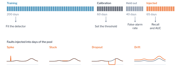
Faults are injected into individual days of the households that do not adopt an EV, so that the day, the kind and the readings of every anomaly are known. A spike multiplies one reading by a factor between two and four and constitutes a point anomaly. A stuck register holds one reading for a block of hours, a dropout replaces a block of readings with zeros, and a drift multiplies the whole day by a factor between 1.4 and 1.8; these three are faults of metering and communication. A meter clock error records the readings of a day ten hours early, the offset between UTC and the time of Victoria, so that the midday export of a PV household appears in the night; it constitutes a contextual anomaly, since its readings are ordinary and only their timing is anomalous. Inverter trips replace the export of two to four spells of one to three half-hours with the household’s demand, as an inverter does when its over-voltage protection disconnects it; they change the occurrence of export and not its timing. Each fault has a counterpart on real networks. Interval records of smart meters carry missing values, repeated readings and errors of time stamp [58], [59], inverters of feeders with high PV penetration disconnect when the voltage at their terminals exceeds the limit of their protection [60], and the drift and the under-recording stand for the metering errors and tampering of non-technical loss [49]. They are injected rather than collected because an operator rarely holds a log of such faults, and labelled sets of real ones are rare and describe other networks and meters, such as the theft labels of a Chinese utility used by Zheng and colleagues [50], [61].
Evaluation with Known Anomalies
A detector fitted on the days of each household is evaluated by the protocol of Figure 10.4. The 365 days of a household are divided at random into 200 training days, 60 calibration days, 40 held-out normal days and a pool of 65 days. The detector is fitted on the training days and its threshold is set on the calibration days. The held-out normal days determine its false-alarm rate, and the days of the pool into which a fault is injected determine its recall.
A measure that does not depend on the threshold is the Area Under the Receiver Operating Characteristic Curve (AUC), the probability that the detector assigns a higher score to an anomalous day than to a normal day. With \(\mathcal{N}\) the scores of the held-out normal days and \(\mathcal{A}\) those of the injected days,
\[ \mathrm{AUC} = \frac{1}{|\mathcal{N}|\,|\mathcal{A}|} \sum_{a \in \mathcal{A}} \sum_{b \in \mathcal{N}} \mathbb{1}\{a > b\}, \tag{10.5}\]
with ties counted as one half. The AUC equals 0.5 for a score unrelated to the anomalies and 1 for a perfect separation.
The AUC, the recall and the false-alarm rate do not depend on the share of anomalous days among those tested. The precision, the share of flagged days that are anomalous, does. With recall \(r\), false-alarm rate \(f\) and a share \(\pi\) of anomalous days, Bayes’ rule gives
\[ \mathrm{precision} = \frac{r \pi}{r \pi + f (1 - \pi)}. \tag{10.6}\]
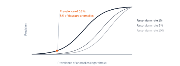
Faults are rare among the days of a population of meters. At a prevalence of 0.1%, a detector with a recall of 90% and a false-alarm rate of 1% flags days of which 8% are anomalous (Figure 10.5). The curve of precision against recall displays this dependence and is therefore more informative than the Receiver Operating Characteristic (ROC) curve when anomalies are rare [62]. The F1 score used below is the harmonic mean of precision and recall, and the false discovery rate of a later section is one minus the precision of a set of flagged meters.
The protocol counts each day once, which avoids a source of overstatement common in the evaluation of detectors on time series. When anomalies occupy segments of consecutive readings, point adjustment counts a segment as detected in full if any one of its readings is flagged [43]. On a year of half-hourly readings containing ten anomalous segments of one to two days, which together make up 4.2% of the readings, a uniformly random score attained a best F1 of 0.079 when each reading was counted and 0.709 under point adjustment (Table 10.3). The difference is due to the adjustment and not to any detection. A result reported under point adjustment must therefore be compared with the score of a random detector under the same adjustment before it is taken as evidence of detection; the evaluations of this part score each day as a whole, without adjustment.
Pitfall: point adjustment
A detection score reported under point adjustment measures the number of segments that contain at least one flagged reading. With long segments and a high rate of flagging, a score unrelated to the anomalies attains a high value. Detectors in this part are therefore evaluated on days, each counted once, with anomalies injected into known days.
Detectors and Their Assumptions
Each family of detectors adopts a different definition of departure, and this definition determines the kinds of anomaly the family detects. All detectors in this section are applied to the 48 readings of a day, each reading standardised by its mean and standard deviation over the training days. Only one of them is parametric: the Mahalanobis distance assumes that normal days follow an elliptical distribution, whose mean and covariance it estimates [13, Sec. 3.2.2]. The others make no assumption on the form of the distribution. Kernel density estimation estimates the density directly from the training days [5], [13, Sec. 16.3], and the reconstruction by principal components is a linear model fitted without a distributional assumption. The families are presented in three groups: those that measure distance or density, those that estimate a boundary, isolate a day or reconstruct it, and a comparison of all of them on the population.
Distance and Density
The Shewhart control limit scores a day by its largest standardised deviation,
\[ s(\mathbf{x}) = \max_{j} \frac{|x_j - \mu_j|}{\sigma_j}, \tag{10.7}\]
and flags the day when the score exceeds three [12]. It assumes that an anomaly is confined to a single reading. Distance-based detectors score a day by its distance to the \(k\)-th nearest training day [3],
\[ s(\mathbf{x}) = \lVert \mathbf{x} - \mathbf{x}_{(k)} \rVert. \tag{10.8}\]
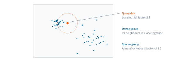
The Local Outlier Factor (LOF) compares the density around a day with the density around its neighbours [4]. With \(\delta_k(\mathbf{o})\) the distance from a training day \(\mathbf{o}\) to its \(k\)-th nearest neighbour, the reachability distance of a day \(\mathbf{x}\) from \(\mathbf{o}\) is
\[ \mathrm{rd}_k(\mathbf{x}, \mathbf{o}) = \max \bigl\{ \delta_k(\mathbf{o}),\ \lVert \mathbf{x} - \mathbf{o} \rVert \bigr\}, \tag{10.9}\]
and the local reachability density of \(\mathbf{x}\) is the inverse of its mean reachability distance from its \(k\) nearest training days \(\mathcal{N}_k(\mathbf{x})\),
\[ \mathrm{lrd}_k(\mathbf{x}) = \Bigl( \frac{1}{k} \sum_{\mathbf{o} \in \mathcal{N}_k(\mathbf{x})} \mathrm{rd}_k(\mathbf{x}, \mathbf{o}) \Bigr)^{-1}. \tag{10.10}\]
The score is the mean ratio of the densities of the neighbours to that of the day,
\[ s(\mathbf{x}) = \frac{1}{k} \sum_{\mathbf{o} \in \mathcal{N}_k(\mathbf{x})} \frac{\mathrm{lrd}_k(\mathbf{o})}{\mathrm{lrd}_k(\mathbf{x})}, \tag{10.11}\]
which is close to 1 for a day as densely surrounded as its neighbours and larger for a day in a sparser region than its neighbours. The detector therefore adapts to regions of different density (Figure 10.6).
The Mahalanobis distance treats the day as a whole. With a robust estimate \(\hat{\boldsymbol{\mu}}\) of the mean and \(\hat{\boldsymbol{\Sigma}}\) of the covariance [11], the score is
\[ s(\mathbf{x}) = (\mathbf{x} - \hat{\boldsymbol{\mu}})^{\top} \hat{\boldsymbol{\Sigma}}^{-1} (\mathbf{x} - \hat{\boldsymbol{\mu}}), \tag{10.12}\]
which under a Gaussian distribution of normal days follows a \(\chi^2\) distribution with \(T\) degrees of freedom, so that a quantile of that distribution provides a parametric threshold. Kernel Density Estimation (KDE) scores a day by the negative logarithm of its estimated density,
\[ s(\mathbf{x}) = -\log \frac{1}{n_{\mathrm{tr}}} \sum_{i \in \mathcal{D}^{\mathrm{tr}}} K_\beta(\mathbf{x} - \mathbf{x}_i), \tag{10.13}\]
where \(K_\beta\) is a Gaussian kernel of bandwidth \(\beta\) and \(n_{\mathrm{tr}}\) the number of training days, a direct estimate of \(p_0\) in Equation 10.3.
Boundaries, Isolation and Reconstruction
The detectors of the previous subsection estimate a distance or a density, from which the level set of Equation 10.3 follows. Boundary methods estimate the level set without the density. Support vector data description encloses the training days, mapped by the feature map \(\Psi\) of a kernel, in the smallest sphere of centre \(\mathbf{a}\) and radius \(R\) that admits slack \(\epsilon_i\) for each day [7],
\[ \begin{aligned} \min_{R,\,\mathbf{a},\,\boldsymbol{\epsilon}}\ & R^2 + C \textstyle\sum_{i} \epsilon_i \\ \text{subject to}\ & \lVert \Psi(\mathbf{x}_i) - \mathbf{a} \rVert^2 \le R^2 + \epsilon_i,\quad \epsilon_i \ge 0, \end{aligned} \tag{10.14}\]
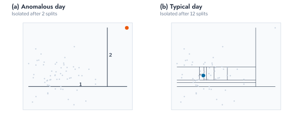
and scores a day by its distance from the centre; with a Gaussian kernel it is equivalent to the One-Class Support Vector Machine (OCSVM) of Schölkopf and colleagues [6]. The Isolation Forest grows random trees, each of which divides the training days at random values of randomly chosen readings, and scores a day by the mean depth \(h(\mathbf{x})\) at which it is isolated [8],
\[ s(\mathbf{x}) = 2^{-\mathbb{E}[h(\mathbf{x})] / c(n_{\mathrm{s}})}, \tag{10.15}\]
where \(c(n_{\mathrm{s}})\) is the mean path length of an unsuccessful search in a binary tree of \(n_{\mathrm{s}}\) points, the size of the sample on which each tree is grown. The score approaches 1 for days that are isolated at a small depth, as Figure 10.7 illustrates. ECOD sums over the readings the negative logarithm of the smaller of the two empirical tail probabilities [9],
\[ s(\mathbf{x}) = -\sum_{j=1}^{T} \log \min \bigl\{ \hat F_j(x_j),\ 1 - \hat F_j(x_j) \bigr\}, \tag{10.16}\]
where \(\hat F_j\) is the empirical distribution function of reading \(j\) over the training days. ECOD assumes that an anomaly is extreme in many readings simultaneously.
Two further families score a day by the error of a model of normal days. A reconstruction-based detector projects a day onto the leading principal directions \(\mathbf{V}\) of the training days and scores the part that the projection does not explain,
\[ s(\mathbf{x}) = \lVert \mathbf{x} - \mathbf{V} \mathbf{V}^{\top} \mathbf{x} \rVert^2, \tag{10.17}\]
the squared prediction error, or Q statistic, of multivariate process monitoring [63]; an autoencoder replaces the linear projection with a non-linear one [18]. The detector assumes that normal days lie close to a low-dimensional subspace, as the principal components of Part 5 showed for daily load profiles. A prediction-based detector scores each reading by the standardised residual of a forecast,
\[ s_t = \frac{|x_t - \hat x_t|}{\hat\sigma_t}, \tag{10.18}\]
where \(\hat x_t\) is a forecast of the reading from its history and from covariates such as temperature, and \(\hat\sigma_t\) the spread of its errors. Residual-based detection is widespread for load data [64], but it requires a forecaster and is therefore taken up with the forecasting methods of Part 8 rather than evaluated here.
Comparison of the Families
The eleven detectors were compared on 40 households of the population, 20 of them with PV, with five days of each fault injected per household (Table 10.4). No detector attained the highest AUC for every fault. The detectors based on distance or density over the whole day attained the highest values. LOF attained the highest mean AUC, 0.952, with 0.976 for spikes, 0.827 for stuck readings and 0.960 for drift, followed by the Mahalanobis distance at 0.933. The reconstruction by five principal components of Equation 10.17 attained 0.924, with 0.962 for drift, which multiplies the part of every reading that lies outside the subspace of normal days. The control limit of Equation 10.7, which responds to a single extreme reading, attained 0.944 for spikes and 0.994 for dropouts but 0.626 for stuck readings, whose held values remain within the normal range of each reading. The detectors based on tail probabilities attained the lowest values. ECOD attained 0.376 for spikes, below the value of 0.5 of a random score, because a single extreme reading contributes one term to the sum of Equation 10.16 over 48 readings, and the remaining terms are determined by the ordinary variation of the day. COPOD and Histogram-Based Outlier Score (HBOS), which have the same construction, attained 0.462 and 0.423. The Isolation Forest attained 0.492 for spikes, since its random splits seldom divide the single reading affected by a spike. A meter clock error displaces the whole day by ten hours, so that the midday export falls in the night and the evening peak in the morning, outside the range of those readings on every training day, and every detector attained an AUC of 1.000 for it; the fault tests whether a representation retains the timing of readings at all and not the power of a detector. Stuck readings were the most difficult fault for every detector, with a highest AUC of 0.827, because a register held at a value attained earlier in the day departs less from the profile than any other fault. The order of the families thus follows from their assumptions, consistent with the dependence on the dataset reported in the comparative studies [16], [17]. For an operator the implication is that the detector follows the fault expected: a density detector such as LOF suits register and communication faults, which place readings where the household has none, whereas a tail-probability detector or an Isolation Forest scores a single spiked reading at or below chance and should not guard against it.
Figure 10.8 shows the same results by fault. The stuck register was the hardest fault for the seven detectors of highest mean AUC, at 0.63 to 0.83, and the spike for three of the remaining four, the Isolation Forest, ECOD and HBOS, which scored it at 0.38 to 0.49, at or below chance; COPOD scored the stuck register lowest, 0.459 against 0.462 for spikes. The ranking of detectors therefore depends on the faults an operator expects, a dependence that the mean over faults conceals.
Figure 10.9 shows one detector on one household’s year, with the threshold calibrated on 60 days that the detector did not see. It flagged 17 of the 20 injected days and 4 of the 40 normal days, a false-alarm rate of 10.0% at the target of 10%. The three drifts it missed scored 1.06 to 1.10 against a threshold of 1.11, in the last quarter of the year: the threshold, not the score, decided the miss. A flag is a decision at a threshold, and a day just below it is no more normal than one just above, which is the reason an operator with a fixed inspection capacity ranks days by score and examines the highest, as the budgets of the last subsection do.
Ensembles of Detectors
A combination of detectors reduces the dependence on the assumption of any single detector. The scores of \(D\) detectors are rescaled to a common range on the training days and combined by their mean, maximum or median, or by the average of maxima. For the last, the detectors are divided at random into \(G\) groups \(\mathcal{G}_1, \dots, \mathcal{G}_G\), and the combined score is
\[ s(\mathbf{x}) = \frac{1}{G} \sum_{g=1}^{G} \max_{\nu \in \mathcal{G}_g} \tilde s_\nu(\mathbf{x}), \tag{10.19}\]
where \(\tilde s_\nu\) is the rescaled score of detector \(\nu\) [20]. The ensemble of six detectors did not exceed its best member (Table 10.5). The median combination attained a mean AUC of 0.930 and the mean combination 0.913, against 0.952 for LOF alone. The maximum and the average of maxima both reproduced the AUC of KDE alone, 0.908, to three decimal places. After rescaling by the range of the training scores, the KDE score exceeded the scores of the other five members on all 100 days with injected drift that were examined, so that it alone determined the maximum. The score of a kernel density estimate increases rapidly for a day distant from all training days, whereas the score of the Isolation Forest is bounded and distance scores increase linearly, so that a rescaling fitted on normal days does not place the scores of anomalous days on a common scale. An ensemble therefore reduces the dependence on an unsuitable member only when its combination rule is robust to a single member, as the median is, and in this population a single detector exceeded every combination.
For an operator who does not know which fault to expect, the implication is to combine detectors by their ranks or their conformal p-values of Equation 10.28 rather than by their raw scores, since a p-value places every member on the same uniform scale under normal behaviour, and to prefer the median to the maximum.
NoteRemark for the machine-learning reader
A detector assumes that normal observations occupy a region of the feature space that a finite sample can describe. In 48 dimensions the distances between observations concentrate, and a distance or density estimated from 200 days is unreliable [22]. The detectors of this chapter work because the normal days of a household lie close to a low-dimensional set, its routine plus noise, so that the principal components of the reconstruction detector capture it in five dimensions. On a population whose normal days vary in more directions the same detectors degrade, which Chapter 2 shows on measured households.
NoteRemark for the power-system reader
Each fault of this chapter has a physical origin that the operator can check: a register that stops updating, a communication link that loses intervals, a current transformer or meter that has drifted from calibration, an inverter that disconnects on over-voltage, and a clock that is set to the wrong time zone. A flag identifies which reading departs from the household’s routine; the origin has to be found on site or in the metering system’s event log.
Representations of a Day
The detectors of the previous sections were applied to the 48 readings of a day. The readings are one representation among several, and the representation determines which departures a detector can observe. This section states this dependence formally, describes the extraction of event-based features, and compares four representations, and the combination of two of them, under two forms of normal variation.
Invariance and Event-Based Features
A representation \(\varphi\) maps the readings of a day to the input of the detector. Let \(g\) be a transformation of a day, either a fault or a form of normal variation. If the representation is invariant to \(g\),
\[ \varphi(g(\mathbf{x})) = \varphi(\mathbf{x}), \tag{10.20}\]
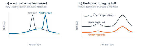
then every detector assigns the transformed day the score of the original day, and no detector on \(\varphi\) can detect \(g\). A suitable representation is therefore invariant to the normal variation of a household and sensitive to its faults. The raw readings are invariant to no transformation and so retain every fault, but they also retain every normal variation. The peak-normalised shape of Part 5 is invariant to the level of demand, and so to under-recording. Summary statistics of level and spread are largely invariant to the timing of the readings. Event features are invariant to variation that does not cross a threshold and to the exact time of an activation within the day. Figure 10.10 illustrates two of these properties.
Event features are designed to possess the invariance that household demand requires. An event is a run of readings beyond a threshold, defined as in Part 5. For a threshold \(\ell\) that a reading falls below, such as an export threshold, the excess at half-hour \(t\) is
\[ e_t = \max \{ 0,\ \ell - x_t \}, \tag{10.21}\]
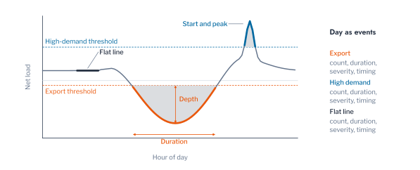
and \(e_t = \max \{ 0,\ x_t - \ell \}\) for a threshold that a reading exceeds. An event is a maximal run of consecutive half-hours with \(e_t > 0\). Three kinds of event are extracted from each day, each with a physical meaning. Export events are runs below \(-0.2\) kW. High-demand events are runs above the household’s own 95th percentile of its training readings, a threshold that adapts to the level of each household as the self-baseline detector does. Flat-line events are runs of readings unchanged from the previous half-hour, the condition that utilities check for a frozen register. For each kind \(c\), the day is summarised by
\[ \boldsymbol{\psi}_c(\mathbf{x}) = \bigl( n_c,\ r_c,\ \bar e_c,\ \max_t e_t,\ \textstyle\sum_t e_t,\ \bar t_c,\ \sigma_{t,c} \bigr), \tag{10.22}\]
where \(n_c\) is the number of half-hours in events, \(r_c\) the number of events, \(\bar e_c\), \(\max_t e_t\) and \(\sum_t e_t\) the mean, largest and summed excess, the last being the severity of Equation 8.1 of Part 6, and \(\bar t_c\) and \(\sigma_{t,c}\) the mean and spread of the hours of the events. The representation of the day concatenates the three vectors, 21 features in place of 48 readings. Part 5 encoded the time of an event on the unit circle because violations occur on both sides of midnight; the events here do not, and the hour is used directly. Figure 10.11 illustrates the extraction.
Representation and Normal Variation
On the population of Equation 10.4, whose normal variation is independent noise around a fixed daily routine, the raw readings attained the highest mean AUC, 0.964 (Table 10.6). A normal day departs from the routine of its household only by noise, so that every fault departs from the routine at some reading, and the raw readings retain every such departure. The peak-normalised shape attained 0.537 for under-recording, close to the value of a random score, as its invariance to level implies, and 0.889 on average. Event features attained the highest AUC for stuck readings, 0.997 against 0.820 for the raw readings, because a frozen register produces a flat-line event that does not occur on a normal day, and they attained 0.986 or more for dropouts, clock errors and inverter trips. They attained 0.625 for under-recording and 0.700 for spikes: a uniform reduction of demand removes some high-demand events without producing new ones, and a spike on a reading that remains below the high-demand threshold produces no event. The combination of event features and summary statistics of level attained 0.926 for under-recording and a mean of 0.930. The summary statistics alone attained 0.640 for inverter trips, since trips leave the deepest export and much of the level of a day unchanged, and the events restored it to 0.986. For an operator, the raw readings suffice while normal days vary only by noise, as here; once timing and level vary normally, as measured households do (Chapter 2), a representation has to ignore that variation, and events are the means of doing so without losing the faults that matter.
Household demand, however, is not noise around a fixed routine. It is the sum of appliance cycles whose times vary from day to day [65]. When randomly timed activations of 1.5 to 3 kW, with a mean of one per household-day, were added to every day, the order of the representations was reversed (Table 10.7). The mean AUC of the raw readings decreased from 0.965 to 0.739, and that of the shape from 0.890 to 0.712, because two normal days with an activation at different hours lie as far apart in these representations as a normal and a faulty day. Event features attained a mean AUC of 0.864, the highest of the four single representations, with 0.997 for stuck readings and for dropouts against 0.542 and 0.667 for the raw readings, because an activation adds a high-demand event of similar duration and depth whatever its time, the invariance of Equation 10.20. The raw readings retained an advantage only for spikes, 0.657 against 0.580, and summary statistics for under-recording, 0.913, the fault that changes the level of a day and not its events. The combination of event features and summary statistics attained the highest mean, 0.890. The suitable representation therefore depends on the form of normal variation. Where normal days differ in the timing of discrete activities, as household demand does, event features retain the faults and discard the variation, and statistics of level complement them for faults of scale. Chapter 2 examines this conclusion on the measured readings of AusNet customers.
Figure 10.12 summarises the two tables. With activations, the mean AUC of the raw readings fell from 0.965 to 0.739 and that of the shape from 0.890 to 0.712, whereas the events fell only from 0.877 to 0.864 and the events with statistics from 0.931 to 0.890. The order of the representations reversed, as Equation 10.20 predicts for features that are invariant to the timing of normal variation. Where the timing of normal behaviour varies from day to day, as it does for households whose routine changes, a detector should therefore be built on events rather than on the readings themselves.
Pitfall: thresholds of events and tied scores
The thresholds that define events are choices of the analyst, and a fault that does not cross a threshold leaves the events of a day unchanged. A threshold derived from the household’s own readings, as for high demand here, adapts to its level, whereas a fixed threshold suits a physical quantity such as export. Event features are also counts, and many normal days have no event of a given kind, so that their features coincide. The resulting tied scores affect the threshold of the detector, as the next section shows.
NoteRemark for the machine-learning reader
A representation decides which departures can be seen, and it does so by discarding information. The shape of a day discards its level, events discard the timing of normal variation, and each choice buys invariance to a variation that is normal at the cost of blindness to a fault that lives in exactly that variation. There is no representation that is best for every fault, only one whose invariances match the variation the population exhibits, so the choice is made from the normal behaviour of the population and then tested against the faults of interest.
NoteRemark for the power-system reader
Household demand varies from day to day in level, with occupancy and temperature, and in timing, with habits and the weather over the PV array, while the aggregate on a transformer varies far less. A representation that is invariant to these variations treats the household as the transformer does, as a source whose total matters more than its shape, and a representation that keeps them treats it as an individual, as a tariff or a hosting study does.
From a Score to a Decision
A score orders the days, and a decision additionally requires a threshold, which determines the false-alarm rate encountered in operation. Several rules for the threshold are in use, and each rests on an assumption about the scores of normal days. This section states these rules, derives the conformal threshold, whose false-alarm rate is known in advance under the weakest of these assumptions, compares the rules on the synthetic population, and extends the conformal threshold to tied scores, to groups of customers and to the simultaneous testing of many meters.
Strategies for a Threshold
The simplest rule fixes the threshold on the scale of the score, as the three-sigma limit of Equation 10.7 does. Such a rule assumes that a score has the same meaning for every household and every detector. The default of most software libraries sets the threshold at the \(1 - \alpha\) quantile of the training scores, where \(\alpha\) is an assumed share of anomalies known as the contamination, and assumes that the training scores represent those of new days. A parametric rule fits a distribution to the scores of normal days. Under a Gaussian assumption, with \(\hat\mu\) and \(\hat\sigma\) the mean and standard deviation of the calibration scores and \(\Phi^{-1}\) the standard normal quantile function, the threshold is
\[ \tau = \hat\mu + \Phi^{-1}(1 - \alpha)\, \hat\sigma. \tag{10.23}\]
A robust rule replaces the mean and the standard deviation with the median and the median absolute deviation, so that anomalies among the calibration days do not inflate the threshold [66], [67],
\[ \tau = \operatorname{med}(s) + 1.4826\, \Phi^{-1}(1 - \alpha)\, \operatorname{MAD}(s), \tag{10.24}\]
where the factor 1.4826 makes the median absolute deviation a consistent estimate of the standard deviation of a Gaussian distribution. An extreme-value rule models only the tail of the scores. Pickands showed that the excesses over a sufficiently high level \(s^{\ast}\) follow approximately a generalised Pareto distribution [27], [68]. With its shape \(\hat\xi\) and scale \(\hat\sigma_{\ast}\) fitted to the \(N_{\ast}\) excesses among the \(n\) calibration scores, the threshold is
\[ \tau = s^{\ast} + \frac{\hat\sigma_{\ast}}{\hat\xi} \Bigl[ \Bigl( \frac{\alpha\, n}{N_{\ast}} \Bigr)^{-\hat\xi} - 1 \Bigr], \tag{10.25}\]
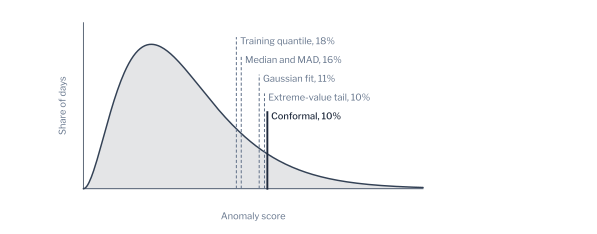
the construction that Siffer and colleagues applied to the detection of anomalies in streams [69]; here \(s^{\ast}\) is the median of the 60 calibration scores, which leaves 30 excesses. Two further rules require information that the preceding rules do not. Where labelled anomalies exist, the threshold may maximise a measure of detection such as F1 on labelled days [70], and where the number of inspections is limited, the meters with the highest scores may be flagged each day up to a fixed budget. The conformal threshold, derived next, assumes only that new normal days are exchangeable with the calibration days. Figure 10.13 compares five of the rules on a skewed distribution of scores, the form that anomaly scores commonly take.
The Conformal Threshold and Tied Scores
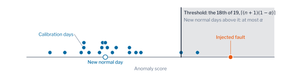
Let \(s_{(1)} \le \dots \le s_{(n)}\) denote the ordered scores of the \(n\) calibration days, which are not used to fit the detector. The conformal threshold at level \(\alpha\) is the order statistic
\[ \tau = s_{(\lceil (n + 1)(1 - \alpha) \rceil)}, \tag{10.26}\]
which is the construction of the trust radius of Part 6 (Equation 6.5) with the anomaly score as the nonconformity score [30], [31]. If a new normal day is exchangeable with the calibration days, the probability that it is flagged satisfies
\[ \Pr\{ s(\mathbf{x}) > \tau \} \le \alpha \tag{10.27}\]
for any detector, as Figure 10.14 illustrates. The guarantee concerns normal days only; the share of anomalous days that exceed \(\tau\) depends on the detector. The level \(\alpha\) is the permitted rate of false alarms per meter and day, so that a population of \(m\) normal meters produces \(\alpha m\) false alarms a day in expectation, the quantity that alarm management limits in operation [53] and that Part 6, Chapter 3 applied to the priorities of live violations. Part 6, Chapter 2 extended the same construction from a coverage to the expected value of a loss by conformal risk control [71]; in the present construction the loss is a false alarm [14, Sec. 14.3].
The seven rules were compared over 20 random splits of 32 households, with LOF as the detector (Table 10.8). The conformal threshold of Equation 10.26 flagged 19.6%, 10.0% and 5.2% of the held-out normal days at targets of 20%, 10% and 5%. The rules fitted to the same calibration days departed from their targets in the directions that their assumptions imply. The scores of LOF are skewed to the right, and the Gaussian rule of Equation 10.23 flagged 15.4% at a target of 20% and 7.7% at a target of 5%, below the target where the Gaussian tail is heavier than that of the scores and above it where the tail is lighter. The median absolute deviation measures the spread of the centre of the distribution and not of its tail, and the rule of Equation 10.24 flagged 27.5%, 20.5% and 16.5%. The extreme-value rule of Equation 10.25 was the closest of the fitted rules, at 20.2%, 11.0% and 6.4%, and exceeded its target at the stricter levels, where the tail was estimated from 30 excesses. The quantile of the training scores flagged 23.8%, 12.8% and 7.1%, because a detector assigns lower scores to the days on which it was fitted than to new days, and a threshold derived from the training scores is consequently too low. Its higher recall, 95.7% of drift days against 93.5% at a target of 10%, is a consequence of the lower threshold and not of better detection. The labelled rule, which maximised F1 on the calibration days and 20 separately injected drift days, flagged 5.4% of normal days and recalled 87.6% of drift days. Its false-alarm rate follows from the share of anomalies among the labelled days, 25% here, rather than from a stated target, and it requires labelled faults of the kind to be detected, which are rarely available. The three-sigma limit on every reading flagged 11.4% of normal days and recalled 68.4% of drift days. A limit of three standard deviations is exceeded by 0.27% of normal readings, but a day comprises 48 readings, and if these were independent the share of days with at least one reading beyond the limit would be \(1 - 0.9973^{48} = 12.2\%\). Of the seven rules, only the conformal threshold maintained its target at every level without labels and without an assumption on the form of the scores.
Figure 10.15 shows the comparison across the three targets. The conformal threshold followed the target at each level, with false-alarm rates of 5.2%, 10.0% and 19.6%. The median and the MAD exceeded it at every level, by 11.5 percentage points at a target of 5%, the training quantile exceeded it by 2 to 4 points, and the Gaussian fit fell below it at 20%, with 15.4%. The recall of drift rose with the false-alarm rate of each rule, so that a rule exceeding its target appears more sensitive only because it accepts more false alarms.
Figure 10.16 sets the rates at the target of 10% against the target itself. The conformal threshold meets it, at 10.0%; the Gaussian fit and the extreme-value tail lie within a point of it; the quantile of the training scores exceeds it by 2.8 points, because the detector scores the days on which it was fitted lower than new days; and the rule based on the median absolute deviation doubles it, at 20.5%, because it measures the spread of the centre of the scores and not of their tail. At 5,000 meters, the difference between a rate of 10% and one of 20.5% is 500 and 1,025 flagged days every day, so an unsuitable rule exhausts the inspection capacity of an operator before any fault is examined.
The bound of Equation 10.27 is exact only in the absence of tied scores, as Part 6 noted for the trust radius. Detectors on count features, such as the event features of Equation 10.22, produce many tied scores, and the threshold then coincides with a value shared by many calibration days. The conformal p-value of a day is
\[ p(\mathbf{x}) = \frac{1 + \#\{ i : s_i \ge s(\mathbf{x}) \}}{n + 1}, \tag{10.28}\]
and the rule \(p(\mathbf{x}) \le \alpha\) is equivalent to that of Equation 10.26. With tied scores, this rule flags fewer normal days than \(\alpha\) permits. The smoothed p-value resolves the ties at random,
\[ p^{U}(\mathbf{x}) = \frac{\#\{ i : s_i > s(\mathbf{x}) \} + U \bigl( 1 + \#\{ i : s_i = s(\mathbf{x}) \} \bigr)}{n + 1}, \tag{10.29}\]
with \(U\) uniformly distributed on \([0, 1]\), and its false-alarm rate equals \(\alpha\) exactly [31]. For the two daily counts of the households with PV, only 4.8% of the calibration scores were distinct (Table 10.9). The conservative p-value flagged 4.9% of normal days at a target of 10% and 2.7% at a target of 5%, so that its threshold was stricter than the target required. The smoothed p-value of Equation 10.29 flagged 9.9% and 4.7%, and at a target of 5% the recall of inverter trips increased from 76.1% to 81.3%, and at a target of 10% from 91.1% to 94.6%. Tied scores therefore leave part of the permitted rate of false alarms unused rather than exceeding it, and the smoothed p-value uses the full rate.
Guarantees for Groups and for Many Meters
The guarantee of Equation 10.27 concerns one meter on one day, averaged over all meters, and a distribution network operator requires two extensions of it: a guarantee within each group of customers, and a bound on the errors among the meters flagged on one day. A single detector fitted on a whole population assigns systematically different scores to groups whose readings vary differently, such as households with and without PV, whose export depends on the weather. A single threshold then maintains the false-alarm rate on average over the groups but not within each group. The Mondrian threshold is calibrated separately within each group \(z\) on the calibration days of that group [31], so that
\[ \Pr\{ s(\mathbf{x}) > \tau_z \mid z \} \le \alpha, \tag{10.30}\]
which is the condition of Equation 6.10 of Part 6 applied to a threshold (Figure 10.17).
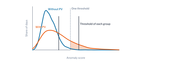
A single LOF detector fitted on the days of all 96 households without an EV, with one threshold at \(\alpha = 0.1\), flagged 7.2% of the normal days of households with PV and 11.3% of those of households without PV (Table 10.10). The readings of the two groups vary differently, so that a single threshold lies at a different quantile of the scores of each group. With one threshold per group, the false-alarm rates were 9.8% and 9.7%, both at the target. A guarantee for each group of customers therefore requires calibration within each group, at the cost of a smaller calibration set for each group.
Figure 10.18 shows the redistribution: the single threshold flagged 7.2% of the normal days of households with PV and 11.3% of those of households without, and the thresholds per group 9.8% and 9.7%.
The second extension arises because a distribution network operator tests all of its meters each day. The threshold of Equation 10.27 bounds the probability that each normal meter is flagged, so that a share \(\alpha\) of the normal meters is flagged each day, and among thousands of normal meters the flagged meters may consist mostly of normal ones. The relevant error rate for the inspection of flagged meters is the false discovery rate, the expected share of flagged meters that are normal. With the p-values of \(m\) meters ordered as \(p_{(1)} \le \dots \le p_{(m)}\), the procedure of Benjamini and Hochberg flags the meters with the \(K\) smallest p-values, where
\[ K = \max \bigl\{ k : p_{(k)} \le \alpha k / m \bigr\}, \tag{10.31}\]
and this bounds the false discovery rate at \(\alpha\) [34], as Figure 10.19 illustrates.
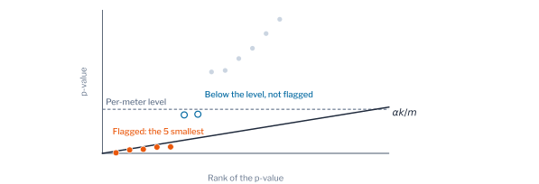
Bates and colleagues showed that conformal p-values satisfy the condition on which this bound rests [33]. All 96 households without an EV were tested on one day, with drift injected into a tenth of them, on each of 20 days (Table 10.11). With 150 calibration days, the per-meter threshold at \(\alpha = 0.1\) flagged 16.2 meters a day, of which 34.8% were normal. The Benjamini-Hochberg procedure flagged 6.4 meters, of which 7.7% were normal, within its bound of 10%, and detected 42.8% of the faulty meters against 94.4% for the per-meter threshold. The procedure therefore trades a lower power for a bounded share of inspections of normal meters. A fixed budget of inspections, the rule of a utility whose field crews can visit a set number of meters each day, flags the meters with the smallest p-values up to that number. With 150 calibration days, a budget of 5 meters had a false discovery rate of 4.0% and a power of 53.3%, and a budget of 20 meters a false discovery rate of 56.2%, because the share of normal meters among those inspected depends on the number of faulty meters, which the budget does not take into account. Its power depends on the size of the calibration set. A conformal p-value cannot be smaller than \(1/(n + 1)\). With 60 calibration days this lower bound, 0.016, exceeds the level \(\alpha k / m\) that Equation 10.31 requires for the ten faulty meters among 96, 0.010, and the power decreased to 13.9%, with a false discovery rate of 10.9%, close to its bound. The simultaneous testing of many meters therefore requires larger calibration sets than a per-meter threshold.
Figure 10.20 shows the two error rates of each rule. The per-meter threshold flagged 16 to 21 meters a day, of which 35% to 45% were normal. The Benjamini-Hochberg procedure held the false discovery rate at 10.9% and 7.7%, near its target, and its power rose from 0.139 to 0.428 with 150 calibration days, because a conformal p-value cannot fall below \(1/(n+1)\). A fixed budget of five inspections attained a comparable false discovery rate with more power on this population, but it carries no guarantee when the share of faulty meters changes.
NoteRemark for the machine-learning reader
The conformal guarantee is marginal and conditional on exchangeability: over the random draw of the calibration days, a new normal day is flagged with probability at most \(\alpha\) [31]. It does not hold for each meter, each season or each group separately, and it fails when the distribution moves; Mondrian thresholds restore it within groups, and Chapter 3 shows it failing under adoption. The guarantee concerns normal days only; the power against faults is not guaranteed and depends on the detector.
NoteRemark for the power-system reader
The false-alarm rate is not a statistical convention but a workload. At a rate of 10% per day, a meter is flagged about three days a month by chance alone, and a feeder of 1,000 meters produces about a hundred flags every day, of which a crew can examine only a few. The rate an operator can accept is set by its inspection capacity, and the rules of the last subsection state how to choose it when the budget, not the rate, is fixed.
Examination of an Alarm
An alarm raises two questions before a meter is inspected: which readings caused the flag, and whether the departure is a fault or a change of the household’s normal behaviour. The examination of a flagged day begins with the readings that contributed most to its score. The Shapley value of reading \(j\) is its mean contribution to the score over all orders in which the readings may be revealed,
\[ \phi_j = \sum_{\mathcal{S} \subseteq \{1, \dots, T\} \setminus \{j\}} \frac{|\mathcal{S}|!\,(T - |\mathcal{S}| - 1)!}{T!} \bigl( v(\mathcal{S} \cup \{j\}) - v(\mathcal{S}) \bigr), \tag{10.32}\]
where \(v(\mathcal{S})\) is the expected score when only the readings in \(\mathcal{S}\) are known. For tree ensembles such as the Isolation Forest, the Shapley values are computed exactly [41], [42]. Figure 10.21 illustrates that the attribution follows the departure from the usual day, which is not necessarily largest where the fault began.
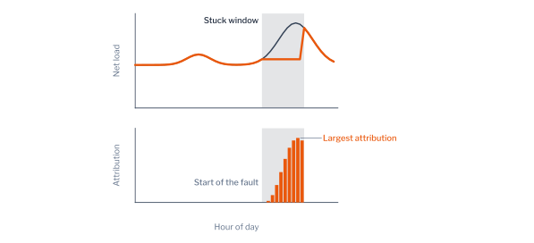
For 200 days with a stuck reading on 40 households, the reading with the largest Shapley value lay inside the stuck window on 51.5% of the days, against 15.1%, the share of the day covered by the window, which is the rate expected of an attribution unrelated to the fault (Table 10.12). Of the five largest attributions, 41.4% lay inside the window. The attribution therefore identifies the faulty hours more often than chance, but not on half of the days, because a held reading alters the relation between readings across the whole day and the Isolation Forest may isolate the day on any reading that separates it. An explanation of this kind guides the examination of a flagged day but does not locate the fault.
Figure 10.22 shows the attribution of one such day across its half-hours. The readings inside the stuck window carry the largest contributions towards the anomalous, as the aggregate result leads one to expect, but readings in the morning and the afternoon contribute as well, because the Shapley values of Equation 10.32 distribute the departure of the score over every reading that the trees of the forest used to isolate the day. For an operator, the plot therefore narrows the examination to the hours that contribute most, and the record of the meter, not the attribution, establishes whether those hours were faulty.
The second question concerns departures that persist. After a household adopts an EV, its readings on every subsequent evening depart from its history. A detector fitted on the earlier days flags these days as anomalies, although no fault has occurred and the normal behaviour of the household has changed. The two situations require different responses, the inspection of a meter in the first case and the refitting of the household’s baseline in the second, and they are distinguished by whether a departure persists (Figure 10.23).
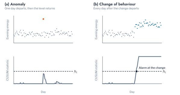
The Cumulative Sum (CUSUM) statistic of Page accumulates the standardised departures of a series \(y_t\) from its reference level \(\mu\), less an allowance \(\kappa\) [36],
\[ S_t = \max \Bigl\{ 0,\ S_{t-1} + \frac{y_t - \mu}{\sigma} - \kappa \Bigr\}, \tag{10.33}\]
and an alarm is raised when \(S_t\) exceeds a level \(h_{\mathrm{c}}\). A single anomalous day increases \(S_t\) once, after which the allowance returns it towards zero, whereas a persistent shift accumulates. Pruned Exact Linear Time (PELT) locates the days of change in a complete series by minimising the cost of a segmentation with a penalty for each change [38]. A Bayesian formulation treats a change as a switch of a hidden state and computes the posterior probability of a change on each day, which also quantifies the uncertainty of its location [72], [14, Sec. 29.3.1] and 29.5.6. A LOF detector calibrated at \(\alpha = 0.1\) on the days before adoption flagged every day after adoption for all 24 households that adopt an EV, in accordance with this argument. The CUSUM statistic with \(h_{\mathrm{c}} = 8\) and \(\kappa = 1\), applied to the evening energy of each household from 18:00 to 22:00, detected every adoption with a median delay of zero days. It also raised 36.6 alarms per year on households whose behaviour did not change, and 14.8 before adoption, because evening energy varies with the season and a fixed reference level treats this variation as a change (Table 10.13). When the evening energy was expressed relative to the mean evening energy of the neighbours on the same transformer, which are subject to the same season, the statistic raised 0.01 alarms per year on unchanged households and none before adoption, and detected every adoption with a median delay of zero days. PELT located the adoption within a median of 2 days on the same relative series. A change of behaviour is therefore detected reliably once the variation that a household shares with its neighbours is removed, a reference that a self-baseline detector of single days does not use.
NoteRemark for the machine-learning reader
An attribution states which readings the detector used to score the day, not which reading caused the fault. The two coincide for a stuck register, whose readings are the departure, and they diverge for any fault that the detector senses through a correlated feature, so an attribution is evidence for a hypothesis to test and not a diagnosis [41].
NoteRemark for the power-system reader
A crew that receives a flag with the readings that raised it knows in which part of the day to look in the meter’s own records, for example the hours of a frozen register, but not which component failed. The attribution shortens the inspection of the record; it does not replace the inspection of the meter.
Further Applications of Anomaly Detection on the Network
The methods of this chapter were illustrated on the readings of household meters, but each of them requires only a set of normal observations, a representation and a score, and the same chain applies wherever a distribution network records a quantity repeatedly. Three further problems of the Low Voltage (LV) network show how the choices of this chapter carry over.
The first is the detection of inverter faults from the export of a PV system. A day of export is represented by its events, the excursions beyond a threshold of Equation 10.21, rather than by its readings, because a fault that interrupts export into short episodes or delays it by an hour changes the number and the timing of the events while leaving the energy of the day nearly unchanged. The invariance of Equation 10.20 then matters in the opposite direction from the meter faults of this chapter: a representation invariant to the timing of the day would make a delayed export indistinguishable from a normal one.
The second is the monitoring of a transformer whose loading drifts as customers adopt PV and electric vehicles. The departure of interest is a persistent change in the distribution of the daily peak rather than an isolated day, and the CUSUM statistic of Equation 12.8, applied to the conformal p-values of Equation 10.28, signals it with a delay that the allowance controls. A drift so detected marks the point at which a model of the transformer, such as the violation patterns of Part 5 or the ranking of Part 6, requires refitting.
The third is the screening of voltage measurements reported by meters, in which a meter whose voltage departs from its neighbours on the same feeder indicates either a fault of the measurement or a connection recorded on the wrong phase or feeder. The neighbours supply the normal observations, the Mondrian threshold of Equation 10.30 sets one threshold per feeder, and the procedure of Benjamini and Hochberg, Equation 10.31, controls the share of false flags among the many meters of a network. Chapter 2 applies these methods to measured readings, and the chapters in preparation apply them to the transformer and the violation event.
Conclusion
This chapter formulated anomaly detection for smart-meter readings as a test of the hypothesis that a day is normal, whose acceptance region is a level set of the density of normal days. A detector approximates the order of that density by a score, and a threshold converts the score into a decision whose false-alarm rate is the type I error of the test. The families of detectors, the representations of a day, the rules for the threshold and the measures of evaluation were each stated formally and evaluated on a synthetic population of 120 households into whose days faults of known kind were injected, by a protocol that counts each day once. Under point adjustment, by contrast, a random score attained an F1 of 0.709, and at a realistic prevalence of faults the precision of a detector depends more on its false-alarm rate than on its recall.
The results on the synthetic population bear on the three questions of the introduction. No detector was superior for every fault. LOF attained the highest mean AUC, 0.952, the control limit detected spikes but not stuck readings, and the detectors based on tail probabilities scored spikes below chance, because a single reading contributes one term to a sum over 48. An ensemble of six detectors did not exceed LOF, and the maximum combination reduced to a single member. The suitable representation of a day depended on the form of normal variation. On days with randomly timed appliance activations, event features attained a mean AUC of 0.864 against 0.739 for the raw readings, and their combination with summary statistics of level 0.890, whereas the raw readings were superior only where normal variation was independent noise around a fixed routine. Of seven rules for the threshold, only the conformal threshold maintained the false-alarm rate at its target at every level without labels and without an assumption on the form of the scores, 10.0% at a target of 10%. A quantile of the training scores flagged 12.8%, a rule on the median absolute deviation 20.5% and the three-sigma rule 11.4%, and an extreme-value fit to the tail came within one percentage point of the target at 10% but exceeded it at 5%. Smoothed p-values used the false-alarm rate that tied scores leave unused, thresholds per group maintained each group of customers at its target, and the Benjamini-Hochberg procedure bounded the share of normal meters among those flagged at 7.7%, against 34.8% for a per-meter threshold, provided that the calibration set was sufficiently large. Shapley values identified the faulty hours on half of the days, more often than chance but not reliably. A change of behaviour, which a detector of single days flags on every subsequent day, was detected by the CUSUM statistic without false alarms once each household was compared with its neighbours.
The limitations are those of a synthetic population. Its readings follow a stated model with a common weather and independent noise, its faults are injected with stated magnitudes, and its households differ only in level, habit, PV and EV adoption. The relative performance of the methods is therefore illustrative. Chapter 2 applies the methods to three measured populations, where the readings contain departures of uncertain cause and some labels exist, such as a register of PV and the price events of a trial, and Chapter 3 to the energy balance of the network, which is not available to a detector of individual meters.
Exercises
- Change \(\alpha\) in the
setupcell to 0.02. How do the false-alarm rate and the recall of Table 10.8 change, and how many of the 60 calibration days lie above the threshold? - Inject a spike of factor 1.5 rather than 2 to 4 into the detector comparison. Which families of Table 10.4 lose the most AUC, and why does the control limit lose less than ECOD?
- Set the share of households with PV to 0.2 in
meters.population. How does the false-alarm rate of the single threshold in Table 10.10 change for each group? - Raise the number of calibration days in the
fdrcell to 250. How do the power of the Benjamini-Hochberg procedure and the smallest attainable p-value change? - Raise the number of calibration days in the
thresholdscell from 60 to 150. How close do the extreme-value rule of Equation 10.25 and the Gaussian rule of Equation 10.23 come to their targets, and why does the conformal threshold not require the larger set? - Raise the high-demand threshold in the
representationscell from the 95th to the 99th percentile of the training readings. How do the AUC of event features for spikes and for stuck readings change, and which property of Equation 10.20 explains the change? - Show that if \(n\) calibration scores and a new score are exchangeable, the threshold equal to the \(\lceil (n+1)(1-\alpha) \rceil\)-th smallest calibration score flags the new score with probability at most \(\alpha\), and compute the exact rate for \(n = 60\) and \(\alpha = 0.1\).
- A random score flags each reading independently with probability \(p\). Derive the probability that point adjustment credits a segment of \(L\) readings, and compute it for \(L = 48\) and \(p = 0.05\); explain from it the F1 of 0.709 that Table 10.3 reports for a random score.
- Show that a limit of three standard deviations on each of 48 independent readings flags \(1 - 0.9973^{48} = 12.2\%\) of normal days, and find the number of standard deviations that gives a rate of 10% per day.