Customers and Connections
Chapter 4 found that a transformer passes through ordered stages of exposure as adoption grows. The stage depends on the rate of adoption and on the transformer, and it does not depend on the load pattern of the households served. The load patterns of Chapter 3 remove the level of demand by peak normalisation. The level is the property of a household to which the thermal limit of a transformer responds.
Two customer-side records therefore remain for an operator that wants its clusters to inform a network decision. The first is the level of demand of each household, which decides how much a household adds to the coincident peak. The second is the phase of each single-phase customer. Voltage is a quantity of one phase, so a study that places a customer on the wrong phase computes the wrong voltage.
Both records are clustering problems, and the chapter treats them with the workflow of Chapters 1 to 4. Each has a unit, a representation, a scaler, a reduction, an algorithm, a number of groups checked against chance, and an outside check that the design has not seen. The first problem keeps the level that Chapter 3 discarded and asks what a group of households can represent in a network study. The second adds the pairwise constraints that Chapter 1 introduced and no later chapter used. A few customers of verified phase supply them, and they are combined with the co-association of Chapter 2 and the prediction sets of Chapter 3. The chapter closes Part 5 with a table of the products of its five chapters against the decisions they serve.
Segments with Level
A segmentation that serves an operator in a network study has to preserve the property to which the study responds. Chapter 3 removed the level of demand because its question was which households use energy at similar times. A household of large demand then joins the group of a household of small demand with the same shape. A study of the thermal limit asks the opposite question. A transformer is loaded by the kilowatts of its customers and not by the shape of their profiles. The segmentation that follows is the clustering of Chapter 3 applied to profiles in kW, with the peak normalisation omitted as the only change of design.
The households are the 342 AusNet households of Chapter 3. Each is described by its weekly profile of 336 half-hourly values in kW, built from the first 180 days of the record. The days that follow remain available to evaluate the groups. The profiles are reduced to two dimensions by t-SNE and grouped by k-means at the number of load patterns of Chapter 3, which is three [1], [2]. A difference between two segmentations then cannot come from a different number of groups. The load patterns are rebuilt in the same way on the first half-year with the peak normalisation. This gives a segmentation of identical design that differs from the first only in the level (Figure 5.1).
The segments are numbered from the lowest mean demand to the highest. Their mean daily profiles in Figure 5.2 share an evening peak and differ mainly in the height of the whole profile. The evening peak is about 0.5 kW in the first segment, 0.9 kW in the second and 1.5 kW in the third. A household of the third segment therefore adds roughly three times the load of a household of the first to the coincident peak. A load pattern built from peak-normalised profiles cannot express this difference.
Verification on a Later Period
A partition is useful for allocation when its groups predict the demand of households in a period they were not built from. The prediction is measured by the share of the variance of a held-out outcome that lies between the groups. For \(G\) groups and \(N\) households, the correlation ratio \(\eta^2\) is the between-group sum of squares over the total. It is positive for any grouping, because a grouping of unrelated households still explains about \((G - 1)/(N - 1)\) of the variance. The bias-corrected form
\[ \varepsilon^2 = \frac{SS_B - (G - 1)\, MS_W}{SS_T} \tag{5.1}\]
removes that chance level. A permutation of the assignment of households to groups gives the null distribution against which the value is judged [3], [4], [5]. The outcomes are the mean demand and the 99th percentile of the demand of each household over the 180 days after the building period. The terciles of the mean demand of the building period serve as the reference that a segmentation of level has to match. Random groups, which explain no variance beyond chance, serve as the lower reference.
The segments that keep the level explained 0.537 of the variance of the mean demand and 0.393 of the variance of the peak demand of the later half-year (Figure 5.3). The chance level was 0.006 and the 95th percentile of the null was 0.018. The terciles explained 0.525 and 0.373, so the clustering adds 0.012 and 0.020 to what the single variable of mean demand supplies. The peak-normalised load patterns explained 0.113 of the mean demand and 0.002 of the peak demand. The second value is indistinguishable from chance (permutation \(p = 0.254\)). A load pattern therefore provides no information on the magnitude of the peak demand of a household, although it describes its timing.
The agreement between the partitions explains the result. The adjusted Rand index between the segments of level and the terciles was 0.771, so the clustering recovers most of the information in the mean demand. Its agreement with the rebuilt load patterns was 0.074 and with the load patterns of Chapter 3 it was 0.071. The two segmentations describe different properties of the same households. An operator that needs the timing of demand uses the load patterns. An operator that needs the size of the load on a transformer uses the segments of level.
Remark: a segmentation is valid for a purpose
A partition has no correctness independent of its use. The same households yield two nearly unrelated partitions when one discards the level and the other keeps it. Each partition is verified against the outcome on which its use depends. Report an outside check with the partition, and prefer the simpler reference, here the terciles, when the clustering does not exceed it by a large margin.
Stability over the Year
An allocation simulated for a year uses a segmentation built from the whole year, and the operator rebuilds the segmentation as data accumulate. The segments built from the first half-year agreed with the demand clusters built from the whole year at an adjusted Rand index of 0.659. This is the persistence of Chapter 3 applied to a design of level, and it shows that the segments change appreciably when six more months are added. A planner should therefore treat the segment of a household as an attribute that is recomputed at each planning cycle. It should not be stored as a property of the customer.
Representative Profiles
A network study cannot replay the readings of every customer of an operator, so it summarises each group of households by one profile. The summary is a prototype of the group, and the two usual choices differ in what they minimise. For a group \(C\) of profiles \(x_i\), the centroid
\[ \bar{x} = \arg\min_{m} \sum_{i \in C} \lVert x_i - m \rVert^2 \tag{5.2}\]
is the mean of the group and the minimiser of the squared error. The medoid minimises the sum of the distances to the members of the group, so it is one of the households [6]. The centroid is smooth and unique, and it is sensitive to outliers. The medoid keeps the shape and the spikes of a real household and depends on the choice of distance. Both are summaries of shape in the sense of Chapter 1. Neither is designed to preserve the quantity on which a network study depends, which is the peak of the sum.
Coincidence of Demand
The households of a group do not peak at the same time, so the peak of their sum is less than the sum of their peaks. For a random subset \(S\) of \(n\) households, the ratio of the first to the second,
\[ c(n) = \frac{\mathbb{E}\left[\max_t \sum_{i \in S} x_i(t)\right]}{n\, \mathbb{E}\left[\max_t x_i(t)\right]}, \tag{5.3}\]
is the coincidence factor. The after diversity maximum demand of distribution planning is the peak per customer that it implies [7]. The factor equals one for a single household and falls towards the value that the mean profile of a large group represents.
The coincidence factor of the AusNet households fell from 0.726 at two households to 0.543 at five, 0.464 at ten and 0.397 at one hundred (Figure 5.4). Most of the fall occurs below twenty households, and the factor changes little beyond them. A mean profile scaled to the number of customers therefore approximates the coincident peak of a feeder or a transformer, but not that of a single connection. At fifty households the coincidence factor was 0.294 in the first segment and 0.471 in the third, where the households share a stronger evening peak (Figure 5.2). A study of a transformer of a hundred customers can use the profile of a group scaled to its size. A study of a feeder of ten customers needs the individual profiles.
The centroid carries the coincident peak of the whole group and none of the spikes of a single household, as Figure 5.5 shows for the three segments. Over the year, the peak of the mean series of a segment was 0.276, 0.405 and 0.464 of the mean peak of its households. The peak of the medoid household was 1.198, 0.984 and 0.734 of it. The squared error of the centroid on the mean daily profiles was lower than that of the medoid for every segment, as the definition requires. The reduction was 7 to 10%, from 0.731 to 0.657 in the first segment and from 7.848 to 7.276 in the third.
Pitfall: a mean profile in place of a peak
A summary that minimises squared error preserves the energy of a group and loses its peak. A network study that assigns the centroid to every customer understates the loading of a single connection. One that assigns a medoid overstates the loading of a large group. Choose the prototype from the quantity on which the study depends, and scale a centroid to the size of the group it represents.
Effect of Who Adopts
The adopters of rooftop Photovoltaic (PV) or an Electric Vehicle (EV) charger are not a random sample of the customers of a network. Adoption varies with building stock and with socio-economic characteristics [8]. A segmentation offers a natural way to describe who adopts. Chapter 4 studied the effect of the rate of adoption with the adopters drawn at random, as in the 25 scenarios of the network it uses. This section holds the number of adopters fixed and varies their allocation. The adopters are drawn at random, from the households of one segment, or from the households of one load pattern. They may also be drawn from whole transformers taken in random order until the number is reached (Figure 5.6).
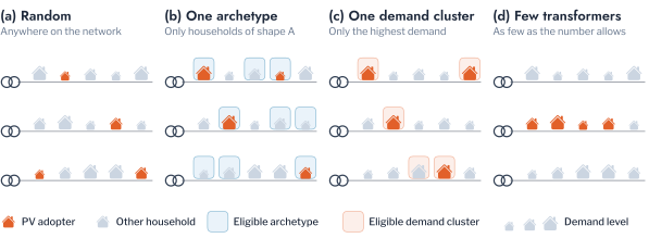
The network is HPK11, with four simulated weeks, one per season, two seeds, and the inverter settings of AS/NZS 4777.2. The allocation uses the segmentation built from the whole year. Adoption was varied from 10 to 25% of the customers, since the smallest segment supplies 28.7% of them (Figure 5.7).
Concentration changed the duration of violations more than any allocation by segment. With PV at 25% of the customers, random allocation produced 859.0 hours of over-voltage over the four weeks. The concentrated allocation produced 1,002.0 hours on 10.5 transformers against 33.5. The effect on the thermal limit was larger, with 1,177.8 hours of overload against 9.8 and 14.5 transformers overloaded against 3. A transformer whose customers all export at midday carries the whole export of its feeder. This is the fully equipped transformer that the stages of Chapter 4 describe. The siting of connections therefore affects this stage more than the selection of customers.
Among the allocations by segment, the level of demand separated the outcomes and the load pattern did not. PV installed only by the households of the segment of highest demand produced 630.8 hours of over-voltage, 26.6% fewer than random allocation. PV installed only by the segment of lowest demand produced 1,051.8 hours, 22.4% more. The three load patterns spanned 760.2 to 904.8 hours, a range of 144.6 hours against 421.0 hours across the three segments. A household of high demand consumes a larger share of its own generation at midday and exports less. The segment of the adopters therefore acts on voltage through its level.
For EV chargers at 25% the under-voltage hours were 56.5, 73.0 and 66.5 for the segments from the lowest demand to the highest, against 59.2 at random. No ordering by level appears, which is consistent with an offset that acts on midday export and not on evening charging.
Remark: stratified allocation as an experiment
Drawing adopters from a stratum is a designed intervention on the composition of the adopters. A survey of existing adopters cannot supply it. It separates the effect of who adopts from the effect of how many adopt, and it is valid only for strata large enough to supply the number of adopters. Each stratum here is a segment of Segments with Level.
Phase Identification
A single-phase customer of an Low Voltage (LV) network is connected to one of the three phases of its feeder. The record of which phase is often wrong, because connections are moved during repairs and reconnections without the record being updated [9], [10]. Every study that depends on the phase of a customer inherits the error. The voltage of a connection is a quantity of one phase. The balance of load between the phases of a transformer cannot be computed without it. The attribution of a violation to the customers that cause it follows the phase on which the customer is placed. A record of phases is therefore a precondition of the network studies of Chapter 4, and it can be recovered from the voltage that each smart meter records.
The identification has been studied as a problem of correlation, of clustering and of optimisation. Meters on the same phase see voltages that move together, and the correlation of their records identifies the phase and the transformer of each customer [9], [11]. Clustering of the voltage series by constrained k-means after a principal component analysis recovered more than 90% of the phases on a feeder of Southern California Edison [12]. Ensembles of partitions combined through a co-association matrix [13] and k-means on feeders with PV [14] have also been used. Comparisons across LV networks showed that the accuracy depends on the share of customers metered and on the quality of the measurements [15], [16]. Model-based formulations that add active and reactive power to the voltage solve the assignment as an integer program [17]. The joint recovery of the phase and the topology from voltage alone is possible under assumptions on the line impedances [18]. The studies differ in the representation of the voltage record, in the unit within which customers are clustered and in the treatment of meter error. These are the choices that this section evaluates.
The evaluation uses the two AusNet urban networks of the book, whose network data record the phase of every single-phase customer (Figure 5.8). The recorded phase is the ground truth for every assignment. The voltage of each customer is solved at its own phase node every half-hour of four weeks from 10 July. Every customer is assigned the measured readings of an AusNet household, and a meter error and a resolution are then added to the solved voltage. No network of real verified phases is available. The results therefore state what the method recovers when the physics is right. They do not state the accuracy on the data of a particular utility.
Voltage as a Signature
The voltage that a meter records is the sum of two components (Figure 5.9). The level falls with the distance of the customer from the transformer, equally on all three phases. It therefore identifies the position of a customer more than its phase. The change from one half-hour to the next is driven by the load on the phase. It moves together for all customers of a phase, scaled by their electrical distance. The correlation between the half-hourly changes of two customers is high when they share a phase and low otherwise, and this is the structure that a clustering can recover.
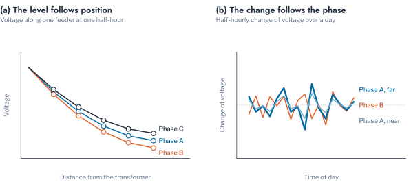
Each meter record is standardised to zero mean and unit variance, so that the product of two records divided by their length is their correlation \(\rho_{ij}\). The affinity \(A_{ij} = (1 + \rho_{ij})/2\) is a similarity between zero and one that spectral clustering uses. The correlation matrix itself is the representation that k-means clusters. The correlation matrix of the meters of one feeder, ordered by phase, shows the contrast (Figure 5.10). The levels of all meters correlate with one another, whereas the half-hourly changes form three blocks.
Representation and Unit
The record is clustered as the level of the voltage or as its half-hourly change. The unit is the customers of one transformer or of one LV feeder, and the algorithm is k-means or spectral clustering. All eight combinations were scored without meter error, over one day and over one week (Figure 5.11). The score is the adjusted Rand index between the three clusters of each unit and the recorded phases. Within an LV feeder the change of voltage recovered the phases exactly after one day with spectral clustering (1.000) and almost exactly with k-means (0.990). The level of voltage within a feeder also scored 0.987 with spectral clustering after one day, since the customers of one feeder differ little in distance.
The unit decides the result for the level. Within a transformer, whose feeders differ in length, the level scored 0.690 with spectral clustering after one day and 0.433 with k-means, whereas the change scored 0.889 and 0.875. A longer record reduced the gap, and a week gave 0.907 and 0.643 for the level and 0.992 and 0.982 for the change. The change of voltage is therefore the representation that does not depend on the geometry of the feeder. A clustering of the level is valid only where the customers of a unit have comparable distances.
Pitfall: clustering a level that encodes another variable
The level of voltage encodes the distance of a customer from its transformer, which dominates the phase when feeders differ in length. A clustering then groups customers by position and agrees with the phases only by chance. Cluster the change of the signal, which removes the position, or restrict the unit to customers at comparable distances.
Accuracy and Length of Record
A meter records voltage with an error and a resolution. The half-hourly change of voltage is small, with a median standard deviation of 0.29% of the voltage in the simulated records. A relative meter error of that size hides the change, and a longer record averages it out. The spectral clustering of the change within each LV feeder was scored for meter errors of 0 to 0.5% and for records of one to 28 days (Figure 5.12).
Without error the phases were recovered exactly at every length of record. At an error of 0.1% one day gave 0.942 and a week 0.999. At 0.2% one day gave 0.795, a week 0.953 and four weeks 0.996. At 0.5%, which is larger than the typical change itself, one day gave 0.239 and four weeks 0.872. A resolution of 1 V in place of 0.1 V reduced the index by up to 0.07 after one day and by less than 0.015 after four weeks. It left the index almost unchanged at 0.5%.
The record length that an operator needs therefore depends on the accuracy of its meters. It is a day for meters of 0.1% error and a month for meters of 0.5%, and the coarser resolution is acceptable. These requirements are the persistence of Chapter 3 applied to a signal of small amplitude. They are consistent with the dependence of accuracy on the time resolution and the duration of the measurements that field trials have reported [10].
Verified Customers and Constraints
A clustering returns three groups with arbitrary names, and a utility needs to know which group is phase A. A few customers of verified phase supply the names. They also supply the constraints that Chapter 1 introduced. Two verified customers of the same phase must share a cluster, and two of different phases must not. Constrained k-means [19] minimises
\[ \sum_{k=1}^{3} \sum_{i \in C_k} \lVert x_i - \mu_k \rVert^2 \quad \text{subject to} \quad z_i = z_j \;\; \forall (i, j) \in \mathcal{M}, \qquad z_i \neq z_j \;\; \forall (i, j) \in \mathcal{C}, \tag{5.4}\]
where \(z_i\) is the cluster of customer \(i\) and \(\mathcal{M}\) and \(\mathcal{C}\) are the must-link and cannot-link pairs. Spectral clustering relaxes the discrete assignment to the leading eigenvectors of the normalised Laplacian of the affinity. The relaxation does not depend on the compactness of the clusters, but it depends on the number of customers of the feeder [20], [21]. A feeder with few customers per phase provides insufficient structure for it, and the unit of clustering is then the transformer.
The three clusterings were compared on the same customers, with one to five verified customers of each phase on every transformer. The verified customers name the clusters by the one-to-one assignment of largest total correlation. Consider a meter error of 0.5% and a week of record. The share of customers named correctly was 0.747, 0.886 and 0.881 with one, three and five verified customers per phase for spectral clustering. It was 0.751, 0.890 and 0.887 for k-means and 0.741, 0.885 and 0.895 for constrained k-means (Figure 5.13). With four weeks the shares were 0.919, 0.955 and 0.959 for spectral clustering, 0.910, 0.943 and 0.942 for k-means, and 0.903, 0.939 and 0.935 for the constrained form.
Three verified customers of each phase on a transformer were sufficient, since a fifth changed the share named correctly by less than 0.01. The constraints from the verified customers provided no improvement over naming the clusters afterwards, because once the correlation structure is clean the verified customers contribute the names and little else. Spectral clustering was the best or equal on every setting at four weeks. It is therefore the simplest adequate method for identifying phase on LV feeders. Constrained k-means remains for feeders on which a verified customer is known to be misrecorded. The cost to the operator is a field verification of three customers of each phase per transformer, which is 9 of the roughly 120 customers of a transformer.
Confidence in an Assignment
A phase assigned to a customer is not equally reliable for every customer. The score of customer \(i\) for phase \(k\) is one minus the correlation of its standardised change with the mean change of the cluster named \(k\). A tenth of the unverified customers, whose phases are verified in the field, calibrate a split-conformal threshold. Each customer then receives the set of phases whose score lies within it. The coverage guarantee is that of Equation 3.20 of Chapter 3, with the exchangeability assumption applied to customers of the same network [22], [23].
The sets of the spectral clustering covered the true phase at the target of 90% on every setting, between 0.883 and 0.929, and their sizes carried the information (Figure 5.14). At an error of 0.5% and a week of record with one verified customer per phase, only 22.9% of the customers received a single phase. The other 77.1% received two or three, so the assignment could not be trusted for most customers. With four weeks the shares were 97.0% with one phase and 3.0% with none. A set of two phases marks a customer for field inspection, and a single phase can be used for operational decisions. The set therefore directs the cost of verification to the customers that need it.
Remark: what crosses a boundary
The method needs the voltage records of the meters, the grouping of customers by LV feeder and the verified phases of a few customers, and it needs no customer’s demand. An operator that cannot release meter data to an analyst can run the clustering locally. It then shares only the thresholds and the accuracy by record length, which carry no customer information.
Transfer to a Second Network
The procedure was fitted on HPK11 and applied unchanged to CRE21, which has 70 transformers and 3,374 single-phase customers against 43 and 5,274 (Figure 5.8). Without meter error the clusters of every feeder agreed with the recorded phases at an adjusted Rand index of 1.000 at a week and at four weeks. At an error of 0.2% the index was 0.953 at a week and 0.988 at four weeks. With three verified customers per phase, 0.975 and 0.982 of the customers were named correctly, and the sets covered at 0.868 and 0.886. At 0.5% the index was 0.674 and 0.833 and the naming accuracy 0.848 and 0.924, with coverage of 0.903 and 0.913.
The results follow those of HPK11, so the requirements of record length and accuracy belong to the physics of three-phase LV feeders and not to the network measured. The coverage at the smaller error was slightly below the target of 0.9. The sets nevertheless remained informative on the second network.
Decision Table
The five chapters of this part produce five kinds of product. Each informs a decision when the records it requires are available and its check has been passed. Table 5.1 states the product, the decision it serves, the records needed and the check that an operator makes before acting.
| Decision | Product | Chapter | Records needed | Check before acting |
|---|---|---|---|---|
| Tariff or engagement of a class of households | Load patterns | 3 | Metered profiles | Verification against chance, set of membership, recomputation each season |
| Which measure a transformer needs, and from what adoption | Violation patterns, groups of cases | 4 | Event records or a network model with profiles | Gate against chance, purity against the decision, transfer to held-out transformers |
| Allocation of new load or generation | Segments that keep the level | 5 | Billed or metered demand | Explained variance of a later period against the terciles |
| Profiles for a network study | Representative profiles scaled to the group | 5 | Metered profiles, a network model | Coincidence factor at the size of the studied group |
| Voltage studies and balance of load | Phase of each customer | 5 | Voltages of the meters, a few verified phases | Prediction set, record length for the meter accuracy, field visit |
| Monitoring of change | Load patterns recomputed with one more group | 3 | Two periods of metered profiles | Recovery of an injected change |
The choice of method within a product depends on the context of the operator, as Table 5.2 states.
| Context | Method | Reason |
|---|---|---|
| Meter error at most 0.2%, a week of voltage records, three phases verified per transformer | Spectral clustering of the half-hourly change within each LV feeder, named from the verified customers | Recovers more than 95% of the phases at the smallest verification cost |
| Meter error of 0.5%, one day of records | Defer the identification, or verify all customers with a set of more than one phase | The change is below the noise, and the sets mark most customers |
| Feeders of fewer than nine customers or without all three phases | Cluster within the transformer on the change of voltage | The spectral relaxation needs enough customers per phase |
| A study of one feeder of ten customers or fewer | Individual profiles | The coincidence factor of a group falls below 0.5 beyond about ten households |
| A study of a transformer of a hundred customers or more | Centroid of the segment scaled to the size of the group | The coincident peak of the group is the quantity needed |
| Allocation of adopters in a scenario study | Segments that keep the level, with concentration on transformers as a separate scenario | Level separates the outcomes, and concentration separates them more |
Further Applications
The workflow of the chapter applies to other customer-side records of an LV network. The same clustering of the half-hourly change of a signal identifies the feeder or the transformer to which a customer is connected. Meters that share a source are more strongly correlated than those that do not. The record of the connection is wrong for the same reasons as the record of the phase. The verified customers of a feeder supply the names, the constraints and the calibration set. The prediction set marks the customers whose connection should be inspected. An operator that installed meters before surveying the network can recover the mapping of customers to transformers from the voltage alone, which every network study of this part requires first.
The segmentation of level applies to the allocation of programmes that act on the peak, such as tariffs of time of use and demand response. The segments of highest demand contribute the most to the coincident peak per customer, and the expected response is proportional to the level. The prototype of a group and its coincidence factor apply to the sizing of a transformer for a new development. The planner then needs the diversified demand of a group of the size of the development. The balance of load between the phases of a transformer follows from the phases identified here. Reassigning customers to equalise the load of the three phases requires their current phases.
In each application the check of the chapter applies. A partition is verified against an outcome on which its use depends. An assignment carries a set that states its confidence. The record length and the accuracy of the meters bound what can be recovered.
Conclusion
The chapter applied the clustering workflow to two customer-side records. Segments built from profiles in kW explained 0.537 of the variance of the mean demand and 0.393 of the peak demand of a later half-year. Load patterns built from peak-normalised profiles explained 0.113 and 0.002. The level that Chapter 3 discarded for good reason is therefore the property that allocation and network studies need. A mean profile carries the coincident peak of a large group, which is 0.40 of the peak of one household at a hundred households. A medoid carries the peak of one household. The profile that represents a group is chosen from the quantity on which the study depends. Concentrating adopters on transformers moved the violations more than any selection by segment.
The phase of a customer was recovered by spectral clustering of the half-hourly change of voltage within each LV feeder. The recovery was exact without meter error, and for meters of 0.2% error the adjusted Rand index was 0.953 at a week and 0.996 at four weeks. Three verified customers of each phase named the clusters, constraints from them added nothing, and a prediction set marked the customers to inspect. The procedure carried to a second network without refitting.
Together with Chapters 3 and 4, these results complete the path of the part from a clustering of customers to a decision on a network. The load pattern informs the engagement of households. The violation pattern and the stage of a transformer inform the measure and its timing. The segment and the phase supply the records that the studies of those decisions require.
Pitfall: reading a clustering of customers as a causal class
A segment describes what households did in a period, and a household can change segment when its occupants or appliances change. An allocation experiment that draws adopters from a segment is an intervention on a description. Its result holds for the households that matched the description when it was built. Recompute the segmentation at each planning cycle and report the stability of the segments with the result.
Scope and limitations
The segments rest on 342 households of one network. The allocation results rest on four weeks of one network with two seeds. The phase results rest on simulated voltages of two networks whose phases are known. The phase method has not been tested with verified field phases, clock offsets between meters or missing readings, and the allocation experiment reaches only 25% of customers.
Exercises
- Show that the centroid of Equation 5.2 is the mean of the group, and that the medoid minimises the sum of Euclidean distances over the members. Give a group of three profiles for which the two differ in the position of their peak.
- Derive the expectation \((G - 1)/(N - 1)\) of the correlation ratio under no association. Use it to show that \(\varepsilon^2\) of Equation 5.1 has expectation zero for \(G\) groups of equal size.
- Take \(n\) independent households whose peaks occur uniformly over \(T\) half-hours and last one half-hour. Give the expected peak of their sum and the coincidence factor of Equation 5.3. Compare it with the measured values at \(n = 5\) and \(n = 20\).
- Show that the leading eigenvectors of the normalised Laplacian of a graph with three connected components are the indicator vectors of the components. Explain why this makes spectral clustering exact when the affinity between phases is zero.
- In the
accuracycell of the companion notebook, add a clock offset of one half-hour to a tenth of the meters. How does the adjusted Rand index of the change of voltage fall, and does the level of voltage recover? - A distribution operator holds the voltage records of 30,000 meters on 400 transformers and the verified phases of 5% of its customers. Design the identification of phase, stating its unit, its representation and the check of each feeder before clustering. Then state the use of the verified customers, the customers referred to field inspection and the statements of this chapter on which the design relies.