Clustering Load Profiles
Smart meters now record the demand of every household at intervals of 15 or 30 minutes. A distribution operator therefore holds a load profile for each customer on a low-voltage feeder. A national population produces millions of such profiles, and no analyst can inspect them one by one. Clustering, a standard tool of smart-meter analytics, answers this problem of scale [1]. It reduces a large population of customers to a small number of recurring consumption patterns on which tariff design, demand response, forecasting and network planning can operate.
The same profiles also matter to the network, because the demand of every household loads the feeder that supplies it. Rooftop solar, residential storage and Electric Vehicle (EV) chargers are connected property by property. A Distribution System Operator (DSO) often learns of their combined effect only when a feeder trips or a transformer overheats. The customer view and the feeder view are two uses of one data set. The first groups customers by what they do, and the second groups them by what they load. This chapter develops the customer view first, because every feeder study starts from a grouping of its customers, and it marks where the feeder view requires something different.
The reduction of a population to a small number of groups has no unique solution, because the result depends on the criterion by which two customers are judged similar. Each household follows its own daily pattern, and the average of the population describes few of them well. Jain’s review of fifty years of clustering research traces the difficulty to the objective. The choice of objective function is a modelling decision and not a property of the data [2]. Four questions have to be settled before a single customer is clustered. The first is which formal criterion makes two customers members of the same group. The second is which features, distance and representation describe a load curve. The third is how the number of groups is chosen and how a grouping is shown to be valid when no labels exist. The fourth is how physical knowledge, such as the feeder to which a customer is connected, shapes the clustering itself.
This chapter answers the first, second and fourth question. It defines clustering formally, selects the features that suit power-system purposes, compares the objective families, examines distance, normalisation and dimension reduction, and shows how network records enter as constraints. For the power-system reader, it shows how to choose features, a normalisation and an objective for a stated purpose, such as tariff design or network planning. It also shows why a method that serves one purpose can fail another. For the machine-learning reader, it states a partition of load curves formally and links each group of features to the physical quantity behind it. It also explains why the records of a distribution operator (feeder, phase, transformer) act as constraints and not as labels. Chapter 2 answers the third question with the validity, stability and selection measures. Each concept is illustrated on a synthetic population of households whose load patterns are known, so that every method can be scored against the truth. Chapters 3 to 6 apply the resulting design to metered data from three utilities.
Clustering Problem
This section states the operator’s problem and defines clustering formally.
A distribution operator uses groups of customers for several decisions, and reviews of smart-meter analytics list tariff design, demand response and network planning among the uses of load profiling [1]. Tariff design needs groups whose members respond similarly to a price signal. Demand-response programmes need groups that can be addressed by one offer. Load forecasting for a population is more accurate when each group is forecast separately, which Kim, Park and Kim use to forecast household demand from clusters of smart-meter series [3]. Energy-efficiency and billing analyses need groups of comparable consumers. Network planning needs groups whose coincident demand loads a transformer in a known way, and hosting-capacity studies need a few representative customers who represent a thousand. Bañales, Dormido and Duro cluster the normalised load shapes of smart-meter customers to segment them by demand-response potential, using only four interpretable features [4]. Chicco’s overview compares the methods for the grouping of load patterns [5].
The decisions differ in what they need from a group, and the difference drives every choice in this chapter. A tariff needs groups that differ in the timing of demand, so that a time-of-use price moves different households in different ways. A transformer study needs the size of demand as well, because the level of demand and not the shape loads the transformer. A programme needs groups that are large enough to justify a separate offer. No single grouping serves all of these decisions. The features, the normalisation and the number of groups are therefore chosen for a stated purpose and not once for the data.
The scale of the problem sets the practical constraints. A utility with a million meters cannot inspect a million profiles, and a grouping that needs a distance matrix of all pairs is already expensive at that size. The cost of each family of methods is compared in the section on objectives, and the representation is kept compact enough for the largest populations. The privacy of the households is a second constraint: a half-hourly profile discloses when a household is at home [6]. A representative profile of many households discloses far less. The minimum size of a group, which Chapter 2 sets from the decision it serves, also limits what a single household reveals.
Let \(\mathcal{I} = \{1, \dots, N\}\) index the meters of a population. A clustering assigns each meter to one of \(K\) groups, and the assignment is a partition.
\[ \mathcal{C} = \{C_1, \dots, C_K\} \tag{1.1}\]
Such that no group is empty (\(C_k \neq \emptyset\)), no two groups share a meter (\(C_k \cap C_l = \emptyset\) for \(k \neq l\)) and every meter belongs to a group (\(\bigcup_{k} C_k = \mathcal{I}\)).
The partition is chosen to minimise an objective that depends on a representation \(\phi\) of each meter and a distance \(d\) between representations.
\[ \mathcal{C}^{\star} = \arg\min_{\mathcal{C}} \; J\bigl(\mathcal{C}; \phi, d\bigr). \tag{1.2}\]
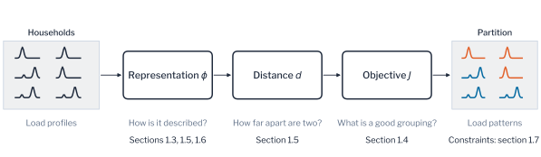
The three ingredients, the representation, the distance and the objective, are separate modelling decisions. The chapter treats the representation first through its features, then the objective families, and then the distance with its normalisation and the reduction of dimension. A partition is hard when every meter belongs to exactly one group, as in Equation 1.1. A soft partition assigns each meter a membership degree to every group, and a mixture model is the standard example. Hard partitions are used throughout the part, because an operator addresses a household as a member of one group. Figure 1.1 shows the three decisions as a path from household profiles to load patterns. The figure is read from left to right. Each box is a decision that the operator can change for a stated purpose without changing the others, and the line under it names the section that treats it.
Two terms are defined here and are used consistently throughout the book. A load pattern is a group of households whose daily profiles are similar under the chosen representation and distance. The representative profile of a load pattern is the profile that represents its members, usually the mean of their profiles. Energy papers often call such a group an archetype. In machine learning the word has another meaning: archetypal analysis finds extreme points on the convex hull of the data and not the centres of groups [7]. The book does not use the word for a group.
Remark: a partition found without labels
A partition in the sense of Equation 1.1 is the customer classification of tariff and planning practice. Every customer has one class, and the classes are found from the readings and not from the billing category. Without labels the objective \(J\) is the only definition of a good grouping. Kleinberg showed that no clustering function satisfies scale invariance, richness and consistency together [8]. The choice of \(J\) is therefore a statement about the application and not a property of the data.
With the problem and the definition in place, the chapter next fixes the notation and the synthetic population on which each concept is demonstrated.
Notation and Population
Consider a population of \(N\) meters, each recording \(T\) readings per day over \(D\) days. The mean daily profile of meter \(i\) is \(\mathbf{x}_i \in \mathbb{R}^{T}\), and its peak-normalised shape is
\[ \mathbf{s}_i = \frac{\mathbf{x}_i}{\max_{t} x_{i,t}}, \tag{1.3}\]
which keeps the timing of consumption and discards its magnitude. A clustering assigns each meter a label \(\lambda(i) \in \{1, \dots, K\}\) and so defines the partition of Equation 1.1 with cluster sizes \(n_k = |C_k|\). Table 1.1 collects the notation of this chapter.
| Symbol | Description |
|---|---|
| \(N\), \(T\), \(D\) | Number of meters, readings per day and days |
| \(\mathbf{x}_i \in \mathbb{R}^{T}\) | Mean daily profile of meter \(i\) |
| \(\mathbf{s}_i \in [0, 1]^{T}\) | Peak-normalised shape of meter \(i\) |
| \(\mathcal{X} \in \mathbb{R}^{N \times D \times T}\) | Meter-by-day-by-reading tensor |
| \(\phi\), \(d(\cdot, \cdot)\) | Representation of a meter and distance between two representations |
| \(K\) | Number of clusters |
| \(\mathcal{C} = \{C_1, \dots, C_K\}\) | Partition; \(n_k = \lvert C_k \rvert\) |
| \(\lambda(i)\) | Cluster label of meter \(i\) |
| \(\mathbf{c}_k\) | Representative profile (centroid) of cluster \(k\) |
| \(J\) | Clustering objective |
The concepts are easier to judge against a population whose structure is known, so each is illustrated on a synthetic one. One hundred and twenty households are drawn from four daily load patterns with evening, morning, daytime and night peaks (Figure 1.3). Each panel shows the normalised profiles of the thirty households of one pattern in grey and their mean in blue. The spread within a pattern can thus be compared with the difference between patterns. Each household has its own size, a daily time shift and multiplicative noise. The size follows a lognormal distribution whose logarithm has a standard deviation of 0.5, which is the spread of the metered AusNet population examined below. Across the thirty populations drawn here, the mean daily profile of a household peaks between 0.18 kW and 5.1 kW, with a median of 1.0 kW. This is the range of a metered low-voltage feeder. To mimic the imperfections of metered data, four meters without a daily routine and one vacant property reporting a constant 0.02 kW are added. The vacant property is removed during data cleaning, which leaves 124 meters.
Every comparison is repeated on thirty populations drawn with different seeds, and a paired Wilcoxon signed-rank test compares methods over the thirty. Because the load patterns are known, a method is scored by how closely its partition reproduces them. The score is introduced here because every later result in the chapter uses it.
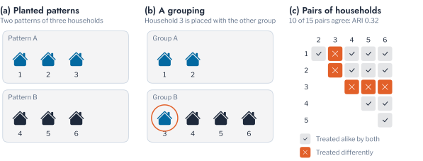
The score is the Adjusted Rand Index (ARI), which compares two groupings of the same households pair by pair. The two groupings agree about a pair when both place it in one group or both place it in different groups. The share of pairs on which they agree is then corrected for the agreement that random groupings would produce by chance. An ARI of 1 means that the two groupings are identical. An ARI near 0 means that the agreement is no better than chance. A negative value means that the agreement is worse than chance. Consider six households, of which the first three belong to one pattern and the last three to another. A grouping that moves the third household into the second group agrees with the truth on 10 of the 15 pairs and scores an ARI of 0.32. A grouping that places every household in one group scores 0, and a grouping that alternates the households between two groups scores \(-0.11\). The score does not depend on how the groups are numbered. A method is not penalised for calling the evening pattern group 3 instead of group 1. Figure 1.2 shows the count for this example. In panel (c) each cell is one of the 15 pairs of households, slate where the two groupings treat the pair alike and orange where they differ. Moving one household spoils the five pairs that contain it, so a few misplaced households lower the score quickly. Chapter 2 gives the formula and develops the other measures of agreement between partitions.
Pitfall: a population that is not homogeneous
A population passed to a clustering algorithm may combine several populations. A vacant property or a faulty meter reports constant or clipped values that look like a distinct pattern but are not household behaviour. Residential and commercial customers are likewise distinct populations for shape-based clustering. The vacant property of the synthetic population is removed before clustering because its readings do not vary.
The population and the score are now fixed. The first ingredient of the definition, the description of each household, comes next.
Profile Features
Every clustering starts from a description of each meter, and the description is a set of features. A record at half-hourly resolution contains 17,520 values per meter and year, and 35,040 at a resolution of 15 minutes. Most of them describe the weather, the calendar or noise and not the behaviour of the household. This section defines the feature map, states which groups of features carry which physical quantity, and measures which of them recover the planted patterns.
A feature map \(\phi : \mathbb{R}^{D \times T} \to \mathbb{R}^{p}\) turns the readings of one meter into \(p\) numbers on which a distance is computed. The design of a feature map is governed by two requirements. The features must vary with the group, so that households of different load patterns differ in them. They must be stable within the group, so that days and seasons of one household do not scatter them. Alelyani, Tang and Liu review feature selection for clustering. Without labels, relevance can only be judged from the structure of the features themselves: their variance, their redundancy and their agreement with a candidate partition [9]. Filter methods rank features by their variance or redundancy before any clustering is run. Wrapper methods score a subset by the quality of the partition it yields. This risks choosing the features that confirm the clusters they produce. A feature that varies widely across households for a reason unrelated to the purpose dominates the distance and hides the structure. Feature selection has to precede the clustering and cannot follow it.
Studies of household load curves support the use of features that describe the shape of the curve. McLoughlin, Duffy and Conlon, Kwac, Flora and Rajagopal, and Haben, Singleton and Grindrod studied household load curves [10], [11], [12]. They showed that clusters built on the shape of a load curve correspond to observable household behaviour and are not statistical artefacts of the algorithm. Bañales, Dormido and Duro segment customers for demand response with only four interpretable features, one of them the entropy of the normalised load shape [4]. A household can also be described by a set of representative daily behaviours and not by one vector. The CROCS framework of Yerbury et al. does so and clusters consumers by the similarity of those sets.1 For tariff design the relevant features describe when demand occurs. For transformer planning they describe how much demand there is and how coincident it is. For anomaly detection they describe what is normal for a household. The same candidate features serve some questions and not others. Three questions recur: grouping households by behaviour, grouping them by loading, and monitoring a household for change. The groups of features defined next are assigned to these questions, and Table 2.1 at the end of the chapter sets the choices out by purpose.
Smart-meter analytics describes a customer by a small number of groups of features, which Wang et al. review [1]. Each group is defined below together with the power-system quantity it carries.
The hour-of-day profile is the mean demand in each hour of the day, by day of the week and by season. It is the most complete description of timing, and its normalised form is the shape of Equation 1.3. The load factor is the ratio of mean to peak demand,
\[ \text{LF}_i = \frac{\bar{x}_i}{\max_t x_{i,t}}, \tag{1.4}\]
computed per day and averaged over days. It is a standard measure of how peaky a customer is and relates directly to the utilisation of a connection. The peak hour \(t^{\star}_i = \arg\max_t \bar{x}_{i,t}\) locates the daily maximum, and the morning-to-evening ratio compares the mean demand between 06:00 and 10:00 with that between 17:00 and 21:00. These three summaries form the shape group, a compact and interpretable description of timing. Figure 1.4 marks them on a daily profile. The calendar group adds the daily peak, the ratio of peak to average demand and the ratio of weekday to weekend energy. The weekday-to-weekend ratio records whether a household has a working routine.
The remaining groups describe the size and the variability of demand and not its timing. The magnitude group holds the mean, spread, maximum, minimum and total of daily energy. The volatility group holds the coefficient of variation of daily energy and its 30-day rolling spread. The trend group holds recent day-on-day changes and the least-squares slope of daily energy. The distribution group holds the skewness, kurtosis and quartiles of daily totals. The autocorrelation group holds the correlation of a series with itself at short lags. It measures the smoothness of the load curve. The lags used here are 0.5 to 6 hours, so the group measures whether demand changes abruptly and not whether the household has a daily routine. Figure 1.4 also marks the mean, spread and slope behind the magnitude, volatility and trend groups on a run of daily totals.
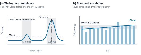
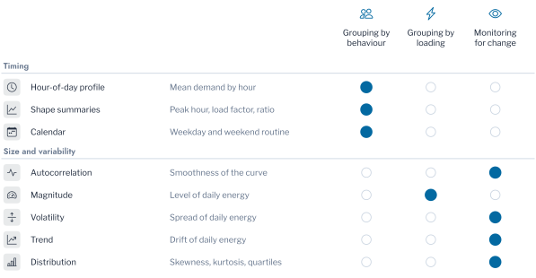
Figure 1.5 assigns each group to the question that it serves. Each row is a group of features, and a filled dot marks a question that the group serves. An operator who needs a grouping by behaviour therefore starts from the groups of timing and not from the size of demand. The groups of timing serve the grouping of households by behaviour. The magnitude group serves the grouping by loading, and the groups of variability serve the monitoring of a household for change.
The relevance of a group can be measured when the patterns are known. Figure 1.6 reports how closely k-means reproduces the planted patterns when it uses each group alone, standardised. Each point is the mean ARI of one group. A point near 1 marks a group that recovers the patterns, and a point near 0 marks one that does not. The score is the mean ARI over thirty populations. The normalised hour-of-day profile recovered the four patterns exactly, with an ARI of 1.000. The shape summaries reached a mean ARI of 0.763, with a lowest value of 0.660, from three numbers per household. The autocorrelation group, at lags of 0.5 to 6 hours, reached 0.704, the calendar group 0.276, and the magnitude, volatility, trend and distribution groups about zero. An ARI of 0.7 to 0.8 means that the grouping places most pairs of households as the planted patterns do but still separates some households from their pattern. A value about zero means that the group describes the households no better than a random assignment.
The reading of these values depends on the construction of the population. The planted patterns differ in the timing of demand only. The groups that describe size and variability cannot recover them, and their ARI near zero is a property of the population and not a general verdict. For the same reason the calendar group, whose main feature is the weekday-to-weekend ratio, carries little information about a population in which no household has a weekday effect. The measurement establishes which of the feature groups carry the timing of demand. The shape of the load serves the grouping by behaviour, and the magnitude group serves the grouping by loading. The volatility, trend, autocorrelation and distribution groups serve the monitoring of a household and the detection of irregular meters. A group that is uninformative about behaviour is informative about loading, and a transformer study needs it.
A few interpretable numbers can therefore replace the full profile when the purpose is the timing of demand. Three shape summaries reached an ARI of 0.763, which is useful when the segmentation must be explained to a regulator or a tariff committee. The full normalised profile remains the choice when the groups must be recovered exactly, and the following sections use it.
Remark: why drop features that are physically meaningful
Kurtosis of daily energy is a well-defined statistic, but it has no direct reading as a property of the behaviour or the connection of a customer. A clustering on it groups households by the form of a distribution and not by what they do. A feature earns a place in a grouping when an engineer can say what a difference in it means for the network or the tariff.
Objective Families
Features define what is compared, and the objective defines what a good group is. Four objective families account for the clustering methods of this part. Each defines a cluster by a different criterion, so the same population can yield different partitions under each [2]. The comparison adds a fifth, the Gaussian mixture, whose objective is a likelihood. Figure 1.7 shows the four families on one toy population before the load profiles return. Each panel draws the boundary that one family finds. The boundaries are regions around centroids, a tree cut at a chosen height, chains of dense points with isolated noise, and a cut through the weakest links. An operator who needs irregular meters flagged therefore needs the family of panel (c), which leaves noise unassigned.
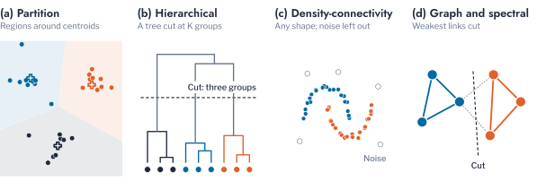
Partition-based objectives (panel (a) of Figure 1.7) place \(K\) centroids so as to minimise the distance of each point to its nearest centroid. For k-means the objective is the within-cluster sum of squares,
\[ J(\mathcal{C}) = \sum_{k=1}^{K} \sum_{i \in C_k} \lVert \mathbf{s}_i - \mathbf{c}_k \rVert^2, \tag{1.5}\]
and each centroid is the mean of its cluster,
\[ \mathbf{c}_k = \frac{1}{n_k} \sum_{i \in C_k} \mathbf{s}_i. \tag{1.6}\]
Lloyd’s algorithm alternates an assignment step, which moves each point to its nearest centroid, and an update step, which recomputes the centroids. Both steps reduce Equation 1.5, and the sequence converges to a local minimum [13], [14]. The seeding of Arthur and Vassilvitskii keeps the expected objective within a logarithmic factor of the optimum [15]. The objective assumes that clusters are compact and of similar spread, because it measures squared distance to a centre. It cannot represent a cluster that wraps around another, and a single distant point pulls a centroid towards itself.
For a load profile the assumption is reasonable when groups are defined by a typical daily rhythm. The centroid is then the representative profile of the group. The distance to it measures how far a household departs from the rhythm. The objective is the default of this part because the representative profile it yields is the object that planning and tariff studies use. Bishop gives the probabilistic reading of the same procedure, in which k-means is the limit of a Gaussian mixture with equal spherical covariances and vanishing variance [16].
Hierarchical objectives (panel (b)) build a tree by repeatedly merging the two closest groups under a linkage rule, and the partition is read off by cutting the tree. Single linkage measures the closest cross-group pair, \(d_{\text{SL}}(G,H) = \min_{i \in G, i' \in H} d_{i,i'}\). Complete linkage measures the farthest pair, \(d_{\text{CL}}(G,H) = \max_{i \in G, i' \in H} d_{i,i'}\). Average linkage measures the mean over all cross-group pairs,
\[ d_{\text{avg}}(G,H) = \frac{1}{n_G n_H} \sum_{i \in G} \sum_{i' \in H} d_{i,i'}. \tag{1.7}\]
Ward’s minimum-variance criterion merges the pair whose union increases the within-cluster sum of squares least. It thus optimises the objective of k-means in a greedy manner [17]. The tree is useful to an operator because it shows how groups nest. Evening-peaking households may split into those with and without an electric vehicle charger, and the tree exposes the split.
The cost of the hierarchical approach is paid in memory and in computation time. The naive algorithm needs the \(N \times N\) distance matrix and \(O(N^3)\) time, reducible to \(O(N^2 \log N)\) with a priority queue. It is impractical for a utility-scale population without sampling. Single linkage chains clusters through intermediate points, and average linkage is sensitive to a few irregular points, as the results below show.
Density-connectivity objectives (panel (c)) dispense with a fixed number of clusters and group points into chains of dense neighbourhoods. In Density-Based Spatial Clustering of Applications with Noise (DBSCAN), a point is a core point when it has a minimum number of neighbours within a radius. It is a border point when it neighbours a core point without meeting that condition itself, and noise otherwise [18]. Clusters are the connected sets of core points together with their border points. Two properties of practical importance follow from this definition. A cluster can take any shape, so DBSCAN recovers the crescent that k-means cannot. Points in sparse regions are labelled noise and not forced into a cluster.
For load data the second property is the more important of the two. A utility population contains meters that belong to no group: a vacant property, a faulty meter, a customer with an unusual operation. A method that must assign every point to a cluster absorbs these meters into the nearest pattern and shifts its representative profile. A density method sets them aside as candidates for inspection. The cost is two parameters, the radius and the minimum number of neighbours. They have no natural value for a profile, and they lose meaning as dimension grows, as the section on dimension reduction shows.
Graph-based and spectral objectives (panel (d)) treat the population as a similarity graph and partition it along its weakest connections. Ng, Jordan and Weiss minimise the normalised cut
\[ \text{Ncut}(S_1, \dots, S_K) = \frac{1}{2} \sum_{k=1}^{K} \frac{\text{cut}(S_k, \bar{S}_k)}{\text{vol}(S_k)}, \tag{1.8}\]
where \(\text{cut}(S_k, \bar{S}_k) = \sum_{i \in S_k, j \notin S_k} w_{ij}\) is the similarity that crosses the cut. The volume \(\text{vol}(S_k) = \sum_{i \in S_k} d_i\) is the total degree within \(S_k\). The relaxed problem is solved with the eigenvectors of the graph Laplacian \(L = D - W\), and k-means is then applied to the rows of the eigenvector matrix [19]. The graph view is natural when similarity is defined by a network and not by a distance, as in the identification of customers on one phase. The method also handles groups that are not convex. The eigendecomposition costs \(O(N^3)\), so spectral methods are the most expensive of the four.
Comparison on Planted Patterns
The families differ in cost, which becomes a selection criterion at utility scale. Partition-based methods cost \(O(NKpI)\) for \(p\) dimensions and \(I\) iterations. Density methods cost \(O(N \log N)\) with a spatial index and \(O(N^2)\) without one. Hierarchical methods cost \(O(N^2 \log N)\) at best, and spectral methods \(O(N^3)\).
Figure 1.8 gives the agreement of seven methods with the planted patterns, in ARI, on the thirty populations. Each point is the mean ARI of one method, coloured by family, and a point at 1 marks a method that recovers the patterns in every population. Partition, Ward, density, spectral and mixture methods recovered the four patterns in almost every population. The mean ARI was 1.000 for five of them and 0.971 for the Gaussian mixture. Average linkage reached 0.709, because a single irregular meter sufficed to merge two groups under the average-distance rule. DBSCAN labelled all four irregular meters as noise in thirty of the thirty populations and Hierarchical Density-Based Spatial Clustering of Applications with Noise (HDBSCAN) in twenty. Every method that must assign each point to a cluster absorbed them into a pattern to which they do not belong.
The choice of objective therefore already decides how irregular meters are treated. If they must be inspected, a density method identifies them as part of the clustering. If a representative profile is the output, a partition method with the irregular meters removed beforehand gives a cleaner centroid. Whether the population contains points that belong to no group must be settled before the objective is chosen. Comparisons on metered data lack the planted truth used here, so they can report only agreement between methods and the values of internal indices. Rajabi et al. compared k-means, fuzzy c-means, hierarchical clustering and self-organising maps on daily load curves and ranked them by validity indices [20]. On the data set of their comparison, hierarchical clustering ranked first and the maps last, and the authors attribute the ranking to that data set and not to the methods. Their comparison contains no density method and does not examine how a method treats irregular curves. Michalakopoulos et al. compared k-means, k-medoids, hierarchical clustering and DBSCAN on nearly 5,000 households of the London population that Chapter 3 also uses [21]. They selected seven groups from the internal indices and rejected k-medoids for its low silhouette. The remaining methods agreed on the largest groups and disagreed on the small ones, and the study does not examine which households a method leaves unassigned. Neither study therefore tests whether the choice of objective changes the treatment of irregular meters. Their results are consistent with the finding of this section, that the methods differ at the edge of the population, but they neither confirm nor refute it.
A Gaussian mixture assumes elliptical groups with soft membership and costs \(O(NKp^2I)\) for \(p\) dimensions. It fails when the groups are not elliptical or a component collapses onto a few points. The simplest adequate method for a population of households is k-means on normalised profiles. A density method run once beforehand removes the meters that belong to no group. A flexible method, such as a Gaussian mixture or a spectral partition, justifies its tuning cost only when the groups are known to be non-spherical. The synthetic population shows no advantage for such a method. All four families rest on a distance between profiles, which the next section examines.
Representation and Distance
Every objective family operates on distances, so the second question of this chapter concerns the representation on which distances are computed and the distance itself. A load curve differs from generic tabular data in two respects. Its magnitude varies by an order of magnitude across households, and its timing can drift from one household to another. This section treats magnitude, then timing, then richer representations.
Normalisation of Profiles
Two households can differ in absolute demand by more than an order of magnitude and still follow the same daily rhythm. A clustering of the mean daily load \(\mathbf{x}_i\) separates households by size, while a clustering of the shape \(\mathbf{s}_i\) separates them by behaviour. The normalisation that turns one into the other is a modelling decision with several forms. Peak normalisation divides by the daily maximum, as in Equation 1.3. Energy normalisation divides by the daily energy, so that a profile sums to one and describes the distribution of demand over the day. The z-score subtracts the mean and divides by the standard deviation, so that a profile has zero mean and unit variance and describes the form of the curve alone. Min-max normalisation rescales each profile to the unit interval. Figure 1.9 shows three households of different size under each form. In the first panel the curves differ in size, and in the other three they coincide, so a distance on any normalised form compares behaviour and not size.
The four forms differ in the property of the profile that they preserve. Peak normalisation keeps the ratio of demand at any time to the peak, which is the quantity that a connection study uses to size a transformer. Energy normalisation keeps the share of consumption at each hour, which is what a time-of-use tariff acts on. The z-score is invariant to both the level and the range of the profile, which serves a comparison of forms but removes the information that the profile is flat. On the planted patterns, the four forms recovered the four patterns exactly, with a mean ARI of 1.000. K-means on the mean daily load reached a mean ARI of 0.222, with a lowest value of 0.097. Removing size matters, and the particular form matters little when timing is the only difference between groups.
The size of the effect depends on how widely household size varies. Figure 1.11 repeats the comparison for log standard deviations of household size from 0.2 to 1.2. The blue line is k-means on the mean daily load, the orange line is k-means on the shape, and the dotted lines mark the spread of the two metered populations. When household sizes are nearly equal, at 0.2, k-means on the mean daily load recovered the patterns exactly. The profiles still differ in timing, and the level adds little scatter. The ARI fell to 0.222 at 0.5, to 0.037 at 0.8 and to 0.007 at 1.2, as size came to dominate the distance. An ARI of 0.222 means that the grouping agrees with the patterns only slightly more than a random grouping would. The shape representation recovered the patterns at every spread. A grouping by load reflects the size of the household once sizes differ widely. A grouping by shape reflects the timing of its use of energy at any spread.
The same distinction holds on metered data, where the planted labels are absent. The partition of mean daily load and the partition of peak-normalised shape agreed with an ARI of 0.016 on the AusNet population of 342 meters. The logarithm of its peak demand has a standard deviation of 0.53, and the peak has 5th, 50th and 95th percentiles of 0.36, 0.91 and 1.92 kW. The agreement was 0.060 on 260 London meters, whose logarithmic spread is 0.81 and whose percentiles are 0.13, 0.42 and 1.86 kW. These spreads correspond to the region of Figure 1.11 in which load clustering has lost the patterns, so the two groupings are nearly independent on real populations. The choice between the two is a choice of question. A study that needs both timing and loading, such as a transformer study, uses both partitions or a representation that retains the level.
Figure 1.10 shows the profiles behind these values. In panels (c) and (f) each cell counts the households in one pair of groups, and a table concentrated on its diagonal would show agreement. In AusNet the groups by load differ mainly in level, and every group by load is spread over all four groups by shape. No cell of the table of households dominates. The one clear association is in London, where eight households with a demand of about 3 kW overnight, falling after 07:00, form a group by load and by shape alike. A tariff built on the groups by load and one built on the groups by shape would otherwise address different households. Chapter 3 studies a cohort of such households, whose overnight peak is the signature of storage heating.
Pitfall: feature scaling is not profile normalisation
Each normalisation makes the distance invariant to one transformation, so the choice states which differences between households the analysis treats as irrelevant. Standardising each column, as is customary for tabular data, does not normalise a profile, because a large household stays large in every column. Divide each profile by its own peak instead (Figure 1.12).
Time Warping
Normalising magnitude leaves the timing of demand untouched. Two households with the same routine may be offset by a fraction of an hour, which a point-by-point Euclidean comparison registers as a mismatch. Dynamic time warping (Dynamic Time Warping (DTW)) addresses the offset in timing. Sakoe and Chiba introduced it for spoken-word recognition, and it computes by dynamic programming the cost of the best monotonic alignment between two series [22]. For \(\mathbf{x} = (x_1, \dots, x_n)\) and \(\mathbf{y} = (y_1, \dots, y_m)\),
\[ D(i, j) = d(x_i, y_j) + \min\{D(i-1, j),\ D(i, j-1),\ D(i-1, j-1)\}, \tag{1.9}\]
with \(D(0, 0) = 0\) and all other boundary cells set to infinity. The DTW distance is \(D(n, m)\). Kotsakos et al. place the measure among the elastic distances for time series and describe its cost, which is quadratic in the series length unless the alignment is constrained [23]. Aghabozorgi, Shirkhorshidi and Wah regard the choice of representation and distance as an open question in time-series clustering [24]. Son, Kim and Kim cluster electricity demand with periodogram-based and autocorrelation-based distances, which compare the frequency content of series and not their alignment in time [25]. Javed, Lee and Rizzo benchmarked eight algorithms with Euclidean, dynamic time warping and shape-based distances over the UCR archive [26]. Sadowska and Gajowniczek found distance-based k-medoids the most robust method on 82 synthetic datasets [27]. Noise degraded the quality of every method more than an increase in the number of classes.
Whether warping improves a clustering depends on whether timing carries information. Figure 1.13 shows the mechanism by which warping removes the timing difference. In panel (a) the vertical lines join readings taken at the same time. In panel (b) the horizontal lines join the readings that warping aligns, which lowers the distance from 2.09 to 0.03. Unconstrained warping can align a morning peak of one household with an evening peak of another when this lowers the total cost. That removes the timing difference that defines the load patterns. A Sakoe-Chiba band limits how far the alignment may stretch, to \(w\) readings on either side of the diagonal. A shift of at most \(w\) readings is then absorbed, and a shift of many hours is not. At half-hourly resolution, a band of two readings treats a household whose routine begins an hour later as the same pattern, and still separates a morning from an evening pattern.
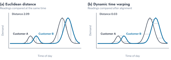
Figure 1.14 shifts the profile of each household by a random time of up to the stated number of hours and clusters the result under three distances, over ten draws. The lines show the mean ARI of each distance, and a line above the others marks the distance that recovers the patterns best at that shift. For shifts of up to one hour, Euclidean distance recovered the patterns exactly, while unconstrained DTW reached a mean ARI of 0.896 (Wilcoxon \(p = 0.031\)). A one-hour band recovered the patterns exactly as well, because it absorbs the shifts that the households have. At shifts of up to 2.5 hours, Euclidean distance (0.789) remained ahead of unconstrained warping (0.652). The difference was not significant over ten draws (\(p = 0.064\)), and the band (0.704) no longer helped. At 4 hours the order reversed: Euclidean distance had degraded to 0.366, unconstrained warping reached 0.504 (\(p = 0.010\)), and the band reached 0.375. Warping harms the grouping while the shifts are small, because it aligns peaks that occur at different times of day and removes the timing difference that defines the patterns. It helps once the shifts exceed what the patterns can tolerate.
The independent benchmark of Paparrizos and Bogireddy supports this reading. Across 128 datasets, no elastic method significantly outperformed the shape-based k-Shape method, and Euclidean-based methods remained a strong baseline [28], [29].
Euclidean distance on time-aligned, normalised profiles is therefore the default for regularly sampled Advanced Metering Infrastructure (AMI) data. Warping, with a band no wider than the expected drift, is reserved for series whose timing drifts by design, such as the output of photovoltaic arrays of different orientation.
Tensor and Diffusion Embeddings
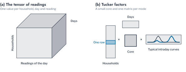
A mean daily profile summarises a season in a single curve. Two further representations retain more of the structure of the readings than the mean profile does. The readings of a population over a season form a three-way array \(\mathcal{X} \in \mathbb{R}^{N \times D \times T}\) indexed by meter, day and reading. Tucker’s decomposition factorises such a tensor into a core tensor and one factor matrix per mode,
\[ \mathcal{X} \approx \mathcal{G} \times_1 \mathbf{A} \times_2 \mathbf{B} \times_3 \mathbf{C}, \tag{1.10}\]
which generalises the matrix factorisation that underlies principal component analysis [30]. The factors have a direct physical reading, in which the columns of \(\mathbf{C}\) are typical intraday curves, and the columns of \(\mathbf{B}\) are typical sequences of days. Each row of \(\mathbf{A}\) gives the loading of one meter on their combinations. Two meters with similar rows have similar daily behaviour, whatever their size. The core \(\mathcal{G}\) records how the three kinds of pattern combine. Figure 1.15 draws the decomposition for the households, the days and the readings of one day of the population. Panel (a) is the tensor of readings, and in panel (b) it is replaced by one matrix per mode and a small core. The highlighted row is the description of one household.
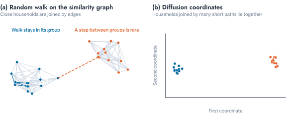
Diffusion maps take a nonlinear route to a similar end. A kernel similarity \(w_{ij}\) between meters defines a Markov transition matrix \(P = D^{-1} W\), which describes a random walk on the graph of meters. The embedding
\[ \Psi_t(i) = \bigl(\lambda_1^t \psi_1(i),\ \lambda_2^t \psi_2(i),\ \dots\bigr) \tag{1.11}\]
scales each leading eigenvector \(\psi_j\) of \(P\) by its eigenvalue raised to the diffusion time \(t\) [31]. The Euclidean distance between two embedded meters approximates their connectivity in the random walk. Meters connected by many short paths lie close together. A long diffusion time smooths over fine structure and leaves the coarse groups. Figure 1.16 shows the walk and the first two coordinates of the population coloured by load pattern. In panel (a) the walk stays inside a group and rarely crosses the dashed link, and in panel (b) the households of one group lie close together.
Both representations recovered the synthetic patterns, with a mean ARI of 1.000 for the Tucker factor and 1.000 for the diffusion map. A richer representation justifies its cost only when the day-to-day behaviour of a household matters. An example is the monitoring of a household for change. For grouping households by a typical day, the normalised mean profile suffices.
Dimension Reduction
Richer representations bring more dimensions, and more dimensions are not necessarily more information. This section states why high dimension harms clustering, describes the common reductions and their assumptions, and gives the pitfalls that apply to load profiles.
As the dimension \(p\) of a representation grows, the distances from a point to its nearest and farthest neighbours become nearly equal. Beyer, Goldstein, Ramakrishnan and Shaft showed that, under broad conditions on the data distribution, the relative contrast between the farthest and the nearest neighbour vanishes as \(p \to \infty\).
\[ \lim_{p \to \infty} \; \frac{d_{\max} - d_{\min}}{d_{\min}} = 0 \quad \text{in probability.} \tag{1.12}\]
Aggarwal, Hinneburg and Keim showed that the effect is stronger for the Euclidean distance than for fractional norms [32], [33]. Aggarwal describes the same effect for outlier detection. Distances to neighbours lose the power to discriminate between normal and abnormal points [34]. Zimek reviews the consequences of this loss of contrast for clustering [35]. Density estimates become unreliable, a fixed radius loses meaning, and a partition can be induced by noise and not by structure. Figure 1.17 shows the contrast of a profile with \(p\) dimensions. It uses the daily profiles of the population, resampled to each dimension, and random vectors of the same dimension. The load profiles keep more contrast than random vectors at every dimension, so a profile of 48 readings can be clustered without a reduction.
A daily load profile has \(T = 24\), 48 or 96 readings, at hourly, half-hourly or quarter-hourly resolution. This is far below the dimension at which contrast vanishes for random data. The profiles are not random, however: neighbouring readings are strongly correlated, so the intrinsic dimension of the profiles is far below 48, and the contrast stays high. The danger arises when representations are stacked, for example 168 weekly hours and 96 seasonal hours in one feature vector. It also arises when the ratio of dimension to sample size grows.
Linear and Nonlinear Reductions
Principal Component Analysis (PCA) finds the orthogonal directions of maximum variance. For the centred matrix of profiles with covariance \(\Sigma\), the components are the eigenvectors of \(\Sigma\), and the variance explained by component \(j\) is \(\lambda_j / \sum_l \lambda_l\) [16], [36]. Shalev-Shwartz and Ben-David show that the principal subspace minimises the reconstruction error among all linear projections of a given dimension [8]. For load profiles the components have a physical reading: the first usually separates daytime from evening demand, and the second separates early from late. The components are dominated by household size unless the profiles are normalised, in which case they describe behaviour. Murphy gives the probabilistic treatment of principal component analysis and the construction of t-Distributed Stochastic Neighbour Embedding (t-SNE) and Uniform Manifold Approximation and Projection (UMAP) [37].
Nonlinear methods trade linearity for local structure, and their purpose differs from that of PCA. t-SNE converts distances to probabilities and places points in two dimensions so that nearby points stay near [38]. The similarity \(p_{ij}\) of two households in the representation is a symmetrised Gaussian kernel whose bandwidth for each household is set by the perplexity, the effective number of neighbours. The embedding places household \(i\) at a point \(\mathbf{z}_i\) of the plane. There the similarity of two households has the heavy tails of a Student distribution with one degree of freedom,
\[ q_{ij} = \frac{(1 + \lVert \mathbf{z}_i - \mathbf{z}_j \rVert^2)^{-1}}{\sum_{k \neq l} (1 + \lVert \mathbf{z}_k - \mathbf{z}_l \rVert^2)^{-1}}. \tag{1.13}\]
The points are placed by minimising the Kullback-Leibler divergence between the two sets of similarities,
\[ \mathrm{KL}(P \,\|\, Q) = \sum_{i \neq j} p_{ij} \log \frac{p_{ij}}{q_{ij}}. \tag{1.14}\]
The divergence penalises placing two neighbours far apart more than placing two strangers close together, so the embedding preserves neighbourhoods and not distances. A large perplexity merges groups and a small one splits a group into fragments, and the default settings of the method do not suit every population [39]. The embedding is therefore a drawing from which only neighbourhoods may be read, and clustering it is a design choice whose effect on the partition has to be tested. UMAP builds a weighted neighbour graph and finds a low-dimensional layout that preserves it [40]. It keeps more of the global arrangement and scales almost linearly with the number of households, which makes it usable as a preparation for clustering on a large population. Pairwise Controlled Manifold Approximation Projection (PaCMAP) was designed to preserve local and global structure together, through three kinds of point pairs [41]. Diffusion maps, treated above, belong to the same family.
Three further nonlinear reductions are used in the chapters that follow. Kernel principal components replace the covariance by a kernel matrix \(\mathbf{K}\) with entries \(k(\boldsymbol{\phi}_i, \boldsymbol{\phi}_l) = \exp(-\gamma \lVert \boldsymbol{\phi}_i - \boldsymbol{\phi}_l \rVert^2)\), centre it as \(\tilde{\mathbf{K}} = \mathbf{H}\mathbf{K}\mathbf{H}\) with \(\mathbf{H} = \mathbf{I} - N^{-1}\mathbf{1}\mathbf{1}^{\top}\), and take the leading solutions of the eigenproblem
\[ \tilde{\mathbf{K}} \boldsymbol{\alpha} = N \lambda \boldsymbol{\alpha} \tag{1.15}\]
as the coordinates [42]. With a linear kernel the solutions are the principal components. UMAP builds a weighted neighbour graph with membership \(v_{il}\) in the feature space. It places the households so that the memberships \(w_{il} = (1 + a \lVert \mathbf{z}_i - \mathbf{z}_l \rVert^{2b})^{-1}\) of the embedding match them, by minimising the cross-entropy
\[ C = \sum_{i \neq l} \left[ v_{il} \log \frac{v_{il}}{w_{il}} + (1 - v_{il}) \log \frac{1 - v_{il}}{1 - w_{il}} \right], \tag{1.16}\]
in which the second term repels households that are not neighbours [40]. PaCMAP minimises a sum over three kinds of pairs, near pairs, mid-near pairs and further pairs, with \(\tilde{d}_{il} = \lVert \mathbf{z}_i - \mathbf{z}_l \rVert^2 + 1\),
\[ L = w_{\mathrm{NB}} \sum_{\mathrm{near}} \frac{\tilde{d}_{il}}{10 + \tilde{d}_{il}} + w_{\mathrm{MN}} \sum_{\mathrm{mid}} \frac{\tilde{d}_{il}}{10^4 + \tilde{d}_{il}} + w_{\mathrm{FP}} \sum_{\mathrm{far}} \frac{1}{1 + \tilde{d}_{il}}, \tag{1.17}\]
where the weights are lowered during the optimisation so that local structure is fixed first and global structure after [41].
Neighbourhood Preservation
The neighbours that a reduction keeps can be counted. Let \(\mathcal{N}_k(i)\) be the \(k\) nearest households of household \(i\) in the feature space and \(\mathcal{M}_k(i)\) its \(k\) nearest households in the reduced space. The preservation of neighbourhoods is a simpler form of the rank-based measures of trustworthiness and continuity [43],
\[ P_k = \frac{1}{N k} \sum_{i=1}^{N} \bigl\lvert \mathcal{N}_k(i) \cap \mathcal{M}_k(i) \bigr\rvert, \tag{1.18}\]
which equals one when every neighbour is kept and falls to \(k / (N - 1)\) for a random embedding. A household whose ten nearest households in the feature space include six that are also among its ten nearest in the plane contributes 0.6 to the mean. On the 124 households of the synthetic population a random embedding would keep 0.08 of the neighbours at \(k = 10\). The first two principal components kept 0.46, PaCMAP 0.58, UMAP 0.60 and t-SNE 0.66. The nonlinear methods keep about a third more neighbours than the linear projection, and all of them lose at least a third of the neighbours of a household. The loss is the reason for the pitfall at the end of this section: an embedding is a display of neighbourhoods and cannot be read as a measurement.
The choice follows the use of the reduction. A representation on which an objective computes distances should keep the geometry that the objective assumes, and a linear projection does so. For load profiles it usually suffices, because neighbouring readings are strongly correlated. A drawing that shows whether groups exist can use a nonlinear layout, from which only the neighbourhoods may be read. A large population that must be clustered in few dimensions is the case for UMAP.
Figure 1.18 places the synthetic population in two dimensions by the first two principal components and by PaCMAP. Both separate the four patterns, and the irregular meters lie between them. Colours and numbers mark the load patterns, and the grey points are the irregular meters. The first preserves distances, so the gap between two groups is a measurement. In the second only the neighbourhoods are meaningful, as the pitfall below explains.
A separate family compresses each series before any clustering, and it matters when a series has many readings, such as a year at half-hourly resolution. Piecewise Aggregate Approximation (PAA) is the simplest of the series reductions. It averages consecutive readings within fixed windows [44], so that 48 half-hourly readings become 12 averages of two hours and the shape of the profile is kept. The discrete Fourier and wavelet transforms describe a series by the coefficients of periodic or localised components and keep the leading ones. The Fourier form suits smooth periodic demand, and the wavelet form suits demand with abrupt changes such as appliance switching. Symbolic Aggregate Approximation (SAX) discretises the PAA series into letters by bands of values, so that a profile becomes a short word that can be compared and indexed quickly [45]. SAX is the coarsest of the three reductions. Every one of them loses sharp peaks, which define a load pattern, and SAX is coarse for differences in amplitude. For a daily profile of 48 readings the reduction is rarely needed, and the normalised profile itself is the better representation.
Autoencoders learn a nonlinear reduction directly from the data, and they need many profiles and careful tuning. Deep Embedded Clustering (DEC) first trains an autoencoder and then adjusts the encoder so that the assignment of each household to a cluster becomes sharper. The embedding and the clusters are thus learned together [46]. Its improved variant, Improved Deep Embedded Clustering (IDEC), keeps the reconstruction loss during the second step, so that the embedding does not distort the structure of the data [47]. Surveys cover deep clustering in general and for time series [48], [49], [50]. Deep clustering justifies its cost only when a large population is available and the linear and symbolic reductions have failed. For every nonlinear method the cost grows with the number of households, from near-linear for UMAP to cubic for a dense diffusion map.
Components to Keep
Dimensionality reduction raises the further question of how many components to keep. A fixed rule, such as keeping the components that explain 90% of the variance, is common but arbitrary. Parallel analysis keeps the components whose eigenvalue exceeds the eigenvalue of the same rank obtained from random data of the same size [51]. Zhu and Ghodsi’s profile-likelihood method locates a change point in the ordered eigenvalues \(\lambda_1 \geq \dots \geq \lambda_p\) without a threshold [52]. The first \(q\) eigenvalues and the remaining \(p - q\) are modelled as two Gaussian groups with a pooled variance. The change point \(q\) maximises
\[ \ell(q) = \sum_{i=1}^{q} \log \mathcal{N}(\lambda_i \mid \mu_1, \sigma^2) + \sum_{i=q+1}^{p} \log \mathcal{N}(\lambda_i \mid \mu_2, \sigma^2). \tag{1.19}\]
Pooling \(\sigma^2\) across both groups prevents the likelihood from diverging as the variance of one group shrinks to zero. On the synthetic population the two rules disagreed (Figure 1.19). The curves are the eigenvalues of the principal components and of the diffusion map, and the vertical lines mark the components that each rule retains. The 90% variance rule retained four components, and the profile-likelihood rule retained two, which together hold 73.4% of the variance. The eigenvalue spectrum has its visible elbow at the number of planted patterns. The elbow of the spectrum and the change point of the profile likelihood are different criteria and are not to be read as one.
The two rules retained four and two components of the same population. A report of a reduction should therefore state the rule that chose the number of components. A rule that is not stated cannot be reproduced on another population, and a fixed share of the variance can hide the elbow of the spectrum. The number of components of a neighbourhood-preserving reduction is a separate choice, because those methods are usually run in two dimensions for display and in more for clustering.
Pitfall: an embedding is a drawing and not evidence
A two-dimensional embedding by t-SNE or UMAP is a drawing and not a measurement. The distances between groups, their sizes and the space between them depend on the perplexity or the neighbourhood size. A partition is therefore judged by the measures of Chapter 2. Fit any scaler or reduction on the training meters only and project the held-out meters through it, since a reduction fitted on all meters lets them influence the representation.
Clustering with Pairwise Constraints
The sections so far use only the readings of the meters. The fourth question asks whether knowledge from outside the meter data can shape the clustering itself. Distance alone carries no record that two customers share a feeder, although a utility usually holds it. This section describes the constraints, shows how a distribution operator uses them, and measures what happens when the records on which they rely are wrong.
Wagstaff, Cardie, Rogers and Schrödl’s constrained k-means makes such knowledge part of the assignment step through two kinds of side information [53]. A must-link constraint requires two points to share a cluster, and a cannot-link constraint forbids it. Assignments that violate either are rejected and not penalised, as Figure 1.20 illustrates. Panel (a) shows the links between customers on two feeders. Panel (b) shows the same customers in profile space, where the must-link pair is far apart and the cannot-link pair is close. The constraints therefore override the distance in both directions. The semisupervised view generalises this to a penalty for violation and to partial labels [54].
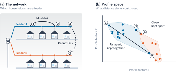
A distribution operator can encode several kinds of knowledge. Customers supplied by the same transformer may be required to share a cluster when the clustering serves a programme for that transformer. Customers on different phases may be forbidden from sharing one when the clustering serves the balancing of phases. Customers on a recorded tariff may be held apart when the clustering estimates the effect of that tariff.
A hard constraint makes the partition depend on records that are themselves uncertain. The recorded phase of a customer is often wrong. A must-link constraint built on a wrong record propagates the error, because must-link constraints are transitive. If \(i\) is linked to \(j\) and \(j\) to \(l\), then \(i\) and \(l\) share a cluster whether or not they are similar. A single wrong link between two groups merges them.
Figure 1.21 measures the effect on the synthetic population. The blue line is constrained k-means and the orange line is k-means without constraints. A share of the must-link pairs, drawn within true patterns, is replaced by pairs across patterns. The ARI of the constrained partition against the planted patterns is recorded against the share of wrong records. Without constraints, k-means stayed at an ARI of 1.000 throughout the experiment. With constraints, the ARI fell to 0.882 at 5% wrong records, 0.772 at 10%, 0.623 at 20% and 0.529 at 30%. The last value lies about half way between a random grouping and the planted patterns. Constraints therefore help only where the records are verified. When the share of wrong records is unknown, a soft constraint with a penalty, or no constraint, is safer. The assignments that the constraints reject are themselves informative. A customer whose readings cannot be placed with its recorded neighbours is a candidate for a recording error.
Remark: why phase records are unreliable
The phase of a single-phase customer is recorded when the service is installed. It changes when crews rebalance a feeder or reconnect after a fault. The record is rarely updated, so a large share of the records on an old network can be wrong. A customer-level record that is wrong by a fixed share is a noise process, and a clustering that uses it must be tested against that noise.
Method Choice by Purpose
The sections above treat features, normalisation, objective, reduction and constraints one at a time. A practitioner makes the choices together for one purpose. Table 2.1 maps the purpose of a grouping to those choices. Each row gives the features that describe the household, the normalisation of the profiles and the objective that forms the groups.
| Purpose | Features | Normalisation | Objective | Notes |
|---|---|---|---|---|
| Tariff design (timing of demand) | Normalised hour-of-day profile, or shape summaries | Peak or energy | k-means | Shape summaries when the result must be explained |
| Transformer and feeder planning | Profile with level retained, magnitude group | None, or peak with level as a second feature | k-means or Ward | Shape alone ignores what loads the transformer |
| Demand-response targeting | Shape and calendar groups | Energy | k-means or k-medoids | Minimum group size set by the programme |
| Detection of irregular meters | Autocorrelation, normalised profile | Peak | DBSCAN or HDBSCAN | Noise label is the output |
| Phase or transformer identification | Voltage series | Z-score | Constrained or spectral | Use only verified records as constraints |
Further Applications
The instruments of this chapter were stated for the daily profiles of household meters, but none of them depends on the object being a household. Any unit of a distribution network that is observed repeatedly can be represented by a curve, compared by a distance and grouped. The questions of features, normalisation, objective and constraints return unchanged. Three further problems of the Low Voltage (LV) network illustrate the transfer.
The first is the grouping of distribution transformers by their loading. The daily loading profile of a transformer is the sum of its customers’ profiles. A clustering of transformers by peak-normalised shape groups them by the composition of their customers, and a clustering by magnitude groups them by utilisation. For transformers, the choice between shape and magnitude becomes the choice between planning by the type of load and planning by the margin to the rating. The feature groups defined above apply to a transformer as to a household, with the load factor reading as the utilisation of the asset.
The second is the grouping of photovoltaic systems by the shape of their generation. Arrays of one orientation and without shading produce nearly the same normalised daily curve on a clear day, while east-facing, west-facing and shaded arrays depart from it in systematic ways. A clustering by shape with the elastic distance of Equation 1.9 separates orientation, which shifts the curve, from shading, which removes part of it. This is the case in which warping is designed to help, because the generation peak drifts by hours with orientation. The households above differ in the time of their peak, which warping would erase. An array that leaves its cluster between years is a candidate for a fault.
The third is the identification of the phase of each customer from the voltage recorded by its meter. Meters on one phase share the voltage variations of that phase. A clustering of the voltage series by correlation, constrained by the must-link relation of customers known to share a phase, recovers the connection. The number of clusters is known in advance, because a low-voltage customer is connected to one of three phases. The instruments of this chapter are used for the opposite purpose to the grouping of households. The agreement with the recorded phases measures how reliable the recovered connection is, not how many groups exist. Chapter 5 develops the method on a physical feeder.
Conclusion
This chapter defined a clustering of load profiles as a partition chosen to minimise an objective over a representation and a distance. It examined each ingredient on a synthetic population of 124 meters whose four load patterns are known. The features that recovered the patterns were those that carry the timing of demand: the normalised hour-of-day profile recovered them exactly, and three shape summaries recovered most of the structure. The features that describe size and variability carry the information that a transformer study needs, and a grouping that uses them answers a different question.
The choice of objective determined how irregular meters were treated, since only density methods set them aside as noise: DBSCAN in every population and HDBSCAN in twenty of thirty. The choice of normalisation determined which question the grouping answers. The partition by load and the partition by shape agreed at an ARI of 0.016 on AusNet and 0.060 on London. Household sizes there vary as widely as in the synthetic populations for which load clustering had lost the patterns. The two are different groupings and not two estimates of one. Unconstrained time warping performed worse than Euclidean distance for shifts of up to one hour and better only at four hours. The load patterns are defined by the time of their peak. An independent benchmark of 84 methods supports this reading. The two rules for retaining components disagreed even on data free of anomalies. Constraints improved a clustering only while the records behind them were correct.
Remark: scope and limitations
The synthetic population is free of anomalies apart from the added meters, and its patterns differ in timing only. The feature and normalisation results therefore state what carries timing and not what matters on every metered population. Constrained clustering was tested on synthetic must-link records and the Sakoe-Chiba band on one range of widths. Findings are rarely tested on a second, independent population, which the chapter addresses by repeating every comparison on thirty populations.
Chapter 2 judges the partitions without labels, tests whether they reproduce under perturbation, and selects the number of groups from the decision that the grouping serves. Chapters 3 to 5 apply the procedure to metered data, where none of the structure is known in advance.
Key findings
Normalised hour-of-day profiles recovered four planted load patterns exactly, and size, volatility and trend features recovered none of them, because the patterns differ in timing only. Clustering on load recovered the patterns when household sizes were nearly equal and lost them as the spread of size grew. The partitions by load and by shape agreed at an ARI of 0.016 on a metered population of 342 meters. Only density-based methods set irregular meters aside as noise. Euclidean distance outperformed unconstrained time warping for small shifts of routine, and warping helped only at a shift of four hours. Wrong must-link records degraded a constrained clustering, so constraints are applied only where records are verified.
Exercises
- Set the spread of household size of the synthetic population to 0.3 and then to 0.65, and repeat the comparison of Figure 1.11. Report where the ARI of k-means on the mean daily load falls below 0.5. Explain from the distance between two households of the same pattern and different size why it falls.
- Add a Sakoe-Chiba band of one hour to the dynamic time warping of Figure 1.14. State the shift at which warping outperforms Euclidean distance and explain why a band of two hours behaves differently from the unconstrained alignment.
- Show that the squared Euclidean distance between two points in \(\mathbb{R}^p\) with independent standard normal coordinates has mean \(2p\) and variance \(8p\). Conclude that the relative contrast of Equation 1.12 vanishes as \(p \to \infty\).
- Derive the update step of Lloyd’s algorithm from Equation 1.5 by setting the derivative of the objective with respect to \(\mathbf{c}_k\) to zero. Show that the assignment step cannot increase the objective.
- A distribution operator holds 40,000 smart-meter profiles and no topology records. It wants to target a demand-response programme at households with an evening peak. Choose the features, the normalisation, the objective and the minimum group size, justify each choice from Table 2.1, and state which choices change if the operator wants to size transformers instead.
Yerbury et al., “CROCS: A Two-Stage Clustering Framework for Behaviour-Centric Consumer Segmentation with Smart Meter Data”, arXiv:2601.10494, 2026.↩︎