Validating Clusters
Chapter 1 defined a clustering of load profiles as a partition and examined the choices that produce one: the features, the normalisation, the distance and the objective. A partition exists as soon as an algorithm has run, but it is not yet a result. Before a distribution operator sizes a transformer or targets a demand-response programme on a group of households, it needs to know whether the groups are well formed. It also needs to know whether they would reappear on another sample of households, and whether they correspond to a real difference in behaviour. No labels exist against which to check any of this, and the number of groups is itself unknown. Published segmentations of smart-meter profiles have been assessed by internal indices and by the correspondence of their clusters with household characteristics [1], [2], [3]. The agreement of an index with the decision that the groups serve is therefore an open question in practice and not only in theory.
This chapter answers the third question of Chapter 1: how a partition is judged without labels. It uses the synthetic population of that chapter (Figure 1.3): four planted load patterns of households, four irregular meters and one vacant property. Each household is described by its peak-normalised shape (Equation 1.3) and grouped by the k-means objective (Equation 1.5). The finding of Conclusion that only density methods set the irregular meters aside is the starting point of the first failure examined below. It first defines the measures of agreement with a known grouping, which score every method on the synthetic population. It then treats internal validity, the stability of a partition under perturbation, and the selection of the number of groups, which combines several indices into one decision. It ends with the external validation of a partition against a change of behaviour that is known to have happened. Each measure is shown on a case where it works and on a case where its assumption fails. A reader can then tell which measure to trust for which question.
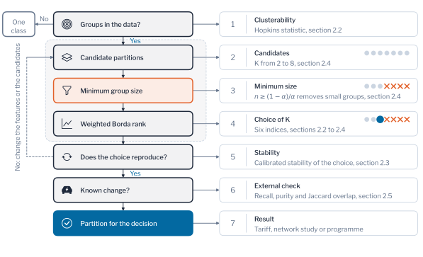
Figure 4.6 shows the order in which the measures of the chapter are used. It is a funnel that narrows the candidate numbers of groups to one. The data are first tested for groups, candidate partitions are built, and the candidates with a group below the minimum size are removed. The weighted rank then chooses among the rest, and the choice is checked for stability and against a known change. The choice is accepted only if it passes the gate of Equation 2.27, a positive excess over structureless data on every check. Otherwise the highest-ranked candidate that passes is taken. The indices of Section 2.2 and the stability measures of Section 2.3 are the inputs of the rank, and stability is checked again for the choice that results. The measures of agreement in Section 2.1 score methods on the synthetic population and are not a step of the path.
Agreement Measures
Chapter 1 scored every method by the Adjusted Rand Index (ARI) against the planted patterns. It introduced the index by counting the pairs of households on which two groupings agree (Figure 1.2). This section states the index formally and compares it with the two other common measures of agreement, the mutual information and the purity. It also shows why a comparison of partitions with different numbers of groups needs a measure that is corrected for chance. The same measures later serve to compare two partitions of real households, when no truth is available.
Let \(U = \{U_1, \dots, U_r\}\) and \(V = \{V_1, \dots, V_s\}\) be two partitions of the same \(N\) households. The overlap of group \(U_i\) with group \(V_j\) is \(n_{ij} = |U_i \cap V_j|\), with row sums \(a_i = \sum_j n_{ij}\) and column sums \(b_j = \sum_i n_{ij}\). Every measure of this section is a function of this table of overlaps. The first measure counts the pairs of households that the two partitions treat alike, together in both or apart in both. The Rand index is the share of the \(\binom{N}{2}\) pairs treated alike.
\[ \text{Rand} = \frac{\text{pairs together in both} + \text{pairs apart in both}}{\binom{N}{2}}. \tag{2.1}\]
The Rand index has a defect that the ARI of Hubert and Arabie corrects [4], [5]. Two unrelated partitions into many groups place most pairs apart in both, so they agree on most pairs by chance alone. The ARI subtracts the number of agreeing pairs expected when the two partitions are drawn independently with the same group sizes. It then divides by the largest value that the difference could take.
\[ \text{ARI} = \frac{\sum_{ij} \binom{n_{ij}}{2} - \dfrac{\sum_i \binom{a_i}{2} \sum_j \binom{b_j}{2}}{\binom{N}{2}}}{\dfrac{1}{2}\left[\sum_i \binom{a_i}{2} + \sum_j \binom{b_j}{2}\right] - \dfrac{\sum_i \binom{a_i}{2} \sum_j \binom{b_j}{2}}{\binom{N}{2}}}. \tag{2.2}\]
The index equals 1 for identical partitions, has expectation zero for independent ones and is negative when the partitions agree less than chance. It does not depend on the labels of the groups, so a method is not penalised for numbering its groups differently from the truth. The six households of Chapter 1 give a table with rows \((2, 1)\) and \((0, 3)\), in which the planted patterns are the rows and the grouping is the columns. Four pairs are together in both partitions and six are apart in both, so the Rand index is \(10/15 = 0.67\). The expected count is \(6 \cdot 7 / 15 = 2.8\) together pairs, and the maximum is \(6.5\), so the ARI is \((4 - 2.8)/(6.5 - 2.8) = 0.32\). The correction removes more than half of the apparent agreement.
The second measure does not count pairs but measures how much knowing the group of a household in one partition reduces the uncertainty about its group in the other. The uncertainty of a partition is its entropy, and the mutual information of two partitions is the reduction in uncertainty that each gives about the other.
\[ H(U) = -\sum_{i} \frac{a_i}{N} \log \frac{a_i}{N} \tag{2.3}\]
\[ I(U, V) = \sum_{i,j} \frac{n_{ij}}{N} \log \frac{N\, n_{ij}}{a_i\, b_j} \tag{2.4}\]
The mutual information is zero when the two partitions are independent, because then \(n_{ij} = a_i b_j / N\) and every logarithm vanishes. It is largest when one partition determines the other. Its value depends on the entropies of the partitions, so the Normalised Mutual Information (NMI) of Strehl and Ghosh divides it by their mean to bring it between 0 and 1 [6].
\[ \text{NMI}(U, V) = \frac{I(U, V)}{\tfrac{1}{2}\bigl[H(U) + H(V)\bigr]}. \tag{2.5}\]
For the six households the NMI is 0.48, so knowing the pattern of a household removes about half of the average uncertainty about its group. A value near 1 would mean that the grouping reproduces the patterns up to relabelling, and a value near 0 that the grouping carries no information about them. The two measures read the same table differently. The ARI is sensitive to the pairs inside large groups, because the number of pairs grows with the square of the group size. The NMI weighs every household by its share of the population. The ARI is corrected for chance, and the NMI is not. With many groups and few households, even independent partitions share some information by chance, so the NMI is biased upwards. Vinh, Epps and Bailey show that this bias can exceed the differences that the measure is meant to detect, and they propose a version corrected for chance [7].
Purity needs a known grouping as reference and assigns each group of the partition \(V\) to the known group \(U_i\) that holds most of its members. It reports the share of households that are assigned correctly.
\[ \text{purity}(V, U) = \frac{1}{N} \sum_{j=1}^{s} \max_i \, n_{ij}. \tag{2.6}\]
Purity is not symmetric, because it asks how pure the groups of one partition are with respect to the other, and the answer changes when the two are exchanged. It is also not penalised for splitting a pattern into several groups, so a partition that places every household in a group of its own has a purity of 1. Its chance level depends on the number of groups, and a random partition into four groups reached 0.33 on the populations used here. It is the easiest of the three to explain to an operator, since it is the share of households that a programme addressed to each group would reach correctly. For the six households it is \((2 + 3)/6 = 0.83\). This is the highest of the three values for the same grouping, because each of its two groups is dominated by one pattern. The three values \(0.32\), \(0.48\) and \(0.83\) are not comparable with one another, because they lie on different scales and correct for chance to different degrees.
Figure 2.2 illustrates the three measures on a known categorisation and a discovered partition of the same objects.
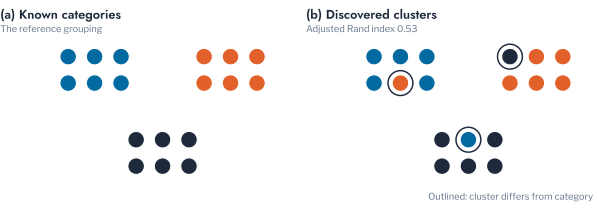
Figure 2.3 compares the three measures on the synthetic populations in two experiments, each averaged over the thirty populations. In the first, a growing share of households is moved to another pattern, which imitates a method that misassigns households. A useful measure falls steadily from 1 to its chance level as the share grows. In the second, the households are assigned to random groups, with the number of groups growing from 2 to 64. This imitates a partition that bears no relation to the truth. A useful measure stays at its chance level whatever the number of groups.
In the first experiment, when 40% of the households had been moved, the ARI had fallen to 0.217, the NMI to 0.232 and the purity to 0.600. At 80% they stood at −0.001, 0.026 and 0.334. An ARI of 0.217 means agreement only slightly better than a random grouping. A purity of 0.600 means that three households in five lie in the group of their own pattern. The NMI lies between 0 and 1, so 0.232 shows that less than a quarter of the information is shared. All three decline together, but they reach different floors. The ARI and the NMI approach zero, whereas purity levels off near one third, the value that a random assignment into four groups reaches by chance.
In the second experiment the measures separate: the ARI stayed at zero for every number of groups, from 0.003 for two groups to −0.002 for eight and 0.000 for 64. The NMI rose from 0.015 for two groups to 0.283 for 64, and the purity rose from 0.302 to 0.629. A partition into many small groups agrees better with any grouping merely because it has more groups. The purity of a group of one household is 1 by construction. Small groups also share information with the known patterns by chance, so neither measure can tell a better partition from one with more groups.
Purity and the NMI therefore cannot compare partitions with different numbers of groups, since both reward a partition for having more of them. An operator who compared a partition into five groups with another into eight would obtain the higher value for the second whatever the data are. The ARI is corrected for chance and can be compared across numbers of groups, which is why Chapter 1 and the later chapters report it.
The three measures complement one another, and none of them suffices alone. The ARI is the main one, because it is corrected for chance and symmetric. The NMI gives an information-based check that does not depend on pairs, and purity answers the operational question for one partition. Xiong and Li review the external measures [8]. Several of them perform poorly when the groups differ in size, which is a reason to report more than one.
Internal Validity Without Labels
The measures of the previous section compare a partition with a grouping that is already known. A utility rarely holds such a grouping, because it has only the readings of its meters and a partition, and it must judge the partition from the readings alone. The first line of evidence is internal: it scores how compact each group is and how far the groups lie from one another. The choice of index matters for load profiles, because the common indices disagree on them and the disagreement depends on the dataset [9], [10]. This section first tests whether the data contain groups. It then defines the indices, shows how they behave across the number of groups, and demonstrates the failure modes that Xiong and Li identify [8] on cases from the low-voltage grid.
Clusterability
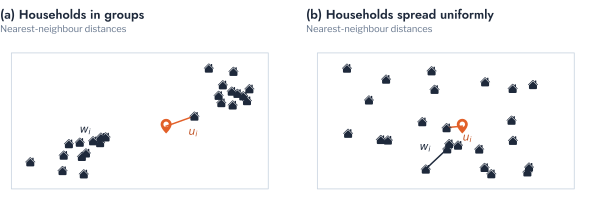
Before any partition is scored, the data themselves can be tested. A partition of data that contain no groups can nevertheless obtain a favourable score from every index that follows. The Hopkins statistic therefore addresses the prior question of whether the data depart from a uniform distribution. It compares two kinds of nearest-neighbour distance [11]. The first, \(u_i\), is the distance from a point drawn uniformly in the range of the data to its nearest household. The second, \(w_i\), is the distance from a sampled household to its nearest other household.
\[ \text{Hop} = \frac{\sum_{i} u_i}{\sum_{i} u_i + \sum_{i} w_i}. \tag{2.7}\]
Values near 0.5 indicate points spread as uniformly as random ones, and values towards 1 indicate groups. The peak-normalised profiles of the synthetic population gave 0.821, against 0.486 for uniform data of the same range. A value near 0.5 would mean that any partition is an arbitrary division of a continuum, and the operator should then treat the population as a single class. Figure 2.4 shows the two distances on households in groups and on households spread uniformly.
The value of 0.821 therefore indicates that the households are far more concentrated in groups than a uniform spread would be. A division of the population into groups is thus justified. It does not indicate how many groups exist or whether they are useful for the decision, which is the subject of the following sections. The statistic depends on the representation, because a population can be uniform in the space of normalised shapes and concentrated in groups in the space of load. It is therefore computed on the representation that the clustering will use, and before any number of groups is chosen. A value near 0.5 leads the operator to treat the population as a single class. The operator then segments it only where the decision requires it, for example by the size of the connection. The subsections that follow define the indices that score a partition once the data are known to contain groups.
The Hopkins statistic shows that the households are concentrated, but not whether the concentrations stand apart from one another. A second test of clusterability asks whether the households fall into disconnected components of a neighbourhood graph. Let \(G_q\) join each household to its \(q\) nearest households, with the edges taken as undirected. Its Laplacian is \(\mathbf{L} = \mathbf{D} - \mathbf{W}\), where \(\mathbf{W}\) is the adjacency matrix and \(\mathbf{D}\) the diagonal matrix of degrees. The multiplicity of the eigenvalue zero of \(\mathbf{L}\) equals the number of connected components of \(G_q\) [12],
\[ \dim \ker \mathbf{L} = \bigl\lvert \{\text{connected components of } G_q\} \bigr\rvert, \tag{2.8}\]
so a spectral method must separate the components before it can find any finer division [13]. A component that survives a large neighbourhood is a group that stands apart from the rest. Ackerman and Ben-David define such separation as a property of the data and not of an algorithm [14].
Figure 2.5 shows the components of the graphs of the thirty synthetic populations. With three neighbours a typical population held five components, and the components recovered the four planted load patterns exactly, at an ARI of 1.000. With five neighbours it held three components and the median ARI fell to 0.71, and with ten neighbours the median ARI was 0.33. The graph was connected in two thirds of the populations at twenty neighbours and in all of them at thirty. The load patterns therefore stand apart only in small neighbourhoods. A graph that is connected at ten neighbours does not prove that there are no groups, because the households of a continuum also form a connected graph. On average 57% of the irregular meters lay in components of five households or fewer at three neighbours and none at five or more. Connectivity thus finds gaps between load patterns and not isolated meters, which the balance and the density-based indices below detect. The operator reads it as evidence of separation, to be tested by the indices and the resampling checks that follow.
Cohesion, Separation and Balance
Every internal index rests on two quantities, cohesion and separation. Cohesion measures how close the households of a group are to one another, and separation measures how far one group lies from another. The indices differ in how they combine the two and in the unit at which they judge a partition: the household, the group or the whole.
Figure 2.6 shows what the first three indices compare.
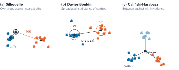
The Silhouette Coefficient (SC) of Rousseeuw judges each household in turn [15]. It compares two mean distances, one within the group and one to the nearest other group. The first, \(a(i)\), is the distance from household \(i\) to the other members of its own group. The second, \(b(i)\), is the distance to the members of the nearest other group.
\[ s(i) = \frac{b(i) - a(i)}{\max\{a(i), b(i)\}} \tag{2.9}\]
The value lies between −1 and 1, and a household with a value near 1 sits well inside its group. A negative value means that the household is closer to another group than to its own, so it is probably misplaced. The SC of a partition is the mean over its households.
The Davies-Bouldin Index (DBI) judges groups instead of households [16]. For each group it finds the neighbour from which it is least separated. This is the neighbour with the largest ratio of the summed spreads to the distance between the centroids. The index is the mean of these worst cases over the groups.
\[ \text{DBI} = \frac{1}{K} \sum_{i=1}^{K} \max_{j \neq i} \left( \frac{\sigma_i + \sigma_j}{d(\mathbf{c}_i, \mathbf{c}_j)} \right) \tag{2.10}\]
Here \(\sigma_i\) is the mean distance of the members of group \(i\) to its centroid \(\mathbf{c}_i\). Lower values indicate better separation, and a single poorly separated pair of groups is enough to raise the index.
The Caliński-Harabasz Index (CHI) judges the partition as a whole [17]. It is the ratio of the variance between groups to the variance within them, in the manner of the \(F\) statistic of an analysis of variance.
\[ \text{CHI} = \frac{SS_B / (K - 1)}{SS_W / (N - K)} \tag{2.11}\]
The between-group term \(SS_B\) is the size-weighted squared distance of the centroids to the overall mean, and \(SS_W\) is the squared distance of every household to its centroid. Larger values indicate groups that are compact and far apart.
These three indices are built from cohesion and separation, and none of them contains a term for the share of the population that a group holds. The balance of a partition supplies it through the normalised entropy of the group sizes [18].
\[ H(\mathbf{p}) = -\frac{1}{\log K} \sum_{k=1}^{K} p_k \log p_k \tag{2.12}\]
Here \(p_k = n_k / N\) is the share of the households that group \(k\) holds. Balance equals one when all groups have the same size and approaches zero when one group holds almost the whole population.
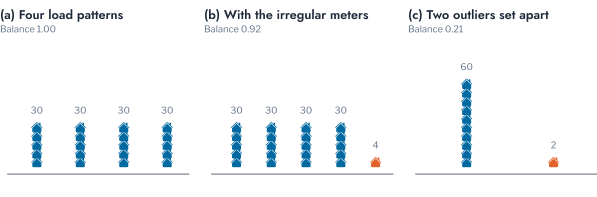
Figure 2.7 shows the balance of three partitions that this chapter meets.
Index Disagreement
Figure 2.8 shows the four indices for the number of groups \(K\) from 2 to 9, on the synthetic population of Chapter 1.
The silhouette rises from 0.440 at two groups to a maximum of 0.724 at five and then falls to 0.569 at nine. The CHI also peaks at five groups, at 367.2 against 273.0 at four. The DBI and the balance point the other way. The DBI is lowest at four groups, at 0.529 against 0.630 at five, and the balance is highest at four, at 0.999 against 0.922. The indices thus divide between five groups, which set the irregular meters apart, and the planted four. The inertia falls from 181.1 to 17.4 without a minimum, so it cannot select a number of groups. A silhouette near 0.7 means that most households lie much closer to their own group than to any other. Four to seven groups all reach it, so the disagreement concerns which number to prefer and not whether groups exist.
Xiong and Li examine how the internal measures respond to monotonicity, noise, differences in density, subclusters, skewed sizes and arbitrary shapes [8]. They find that no measure is robust to all of them. The disagreement above shows two of these failures, the monotone fall of the inertia and the effect of skewed sizes, and skewed sizes are the simpler to isolate.
Figure 2.9 shows 62 points: 60 drawn from one Gaussian cloud and two placed far from it. Treating the two distant points as a cluster of their own gave a silhouette of 0.921, a CHI of 483.6 and a DBI of 0.069. A split of the main cloud gave 0.166, 7.6 and 1.333, so all three separation measures preferred the partition that isolates two points. A silhouette of 0.921 means that every point lies far closer to its own group than to the other. A DBI of 0.069 means that the spread of each group is a small fraction of the distance between the groups. The CHI has no fixed scale and is read only against the 7.6 of the competing partition. Balance alone distinguished the two partitions, at 0.206 for the isolated pair against 0.999 for the split.
The four irregular meters of Chapter 1, which have no daily routine, form a group of this kind. Clustering methods for outlier detection treat such small groups as outliers [19]. A partition that sets them aside as a cluster separates them perfectly. Chapter 1 showed, however, that a density method labels them as noise and not as a pattern. The partition scores highly on every separation index but cannot serve a tariff, because the group is too small to address and too heterogeneous to describe. Balance is a diagnostic and not a proof. A genuine minority pattern lowers it too, as the section on selecting the number of groups shows.
The next subsections show a failure of an index that assumes compact groups and then examine the density-based and model-based indices.
Groups of Unusual Shape
The SC and the DBI measure distance to a centre, so they assume compact groups. Figure 2.10 shows two crescents of points. The planted grouping, which follows the crescents, had an SC of 0.326, while the grouping of k-means, which crosses them, had 0.487. The Density-Based Cluster Validity (DBCV) of Moulavi et al. compares the sparseness of the density inside each group with the density separation between groups [20]. It uses minimum spanning trees and so does not assume compact groups. It scored the planted grouping at 0.477 and the grouping of k-means at −0.811. The index lies between −1 and 1, and a negative value means that the sparseness inside the groups exceeds the separation between them. The density-based index therefore ranks the two groupings in the opposite order from the silhouette, and in the order of the planted structure.
Load profiles take such shapes, because a small change in the timing of demand changes a profile only slightly. A household whose evening peak occurs a little later has a profile close to that of a household with an earlier peak. A population whose peak times spread continuously from 17:00 to 21:00 therefore forms a chain of similar profiles whose ends differ. In the space of profiles the chain is a curve, and a method that assumes compact groups divides it into compact pieces, which the separation indices score highly. A density-based index is appropriate for groups of this kind. Its cost is computation, which grows quickly with the number of households, so it is reserved for the few candidate partitions that remain.
Density and Model-Based Indices
The indices above measure distance to a centre or between centres. Two further families of indices do not make that assumption. Density-based indices judge a group by the paths that connect its members, and the DBCV of the previous subsection belongs to this family. The density silhouette is the silhouette of Equation 2.9 computed on shortest-path distances through a graph of nearest neighbours, so a crescent is compact along its length. The local cores index of Cheng et al. replaces each group by the points of locally highest density [21]. It divides the smallest distance between the cores of different groups by the mean distance between the cores of one group.
Model-based indices judge how well a simple rule separates the groups. The mean-max index divides the smallest distance between two group centres by the mean over the groups of the largest distance from a member to its centre. The Fisher index projects each pair of groups on the direction that separates them best. It reports one minus the share of pairs whose projections overlap enough to suggest that the two groups should merge.
Figure 2.11 shows these indices and the DBCV on the synthetic population. The density silhouette was largest at four groups, at 0.830 against 0.781 at five. The DBCV rose to 0.736 at five groups and was undefined beyond it. The local cores index preferred three groups, at 2.659, and the mean-max index preferred seven, at 7.155 against 7.136 at five. The Fisher index equalled 1.000 for two, three and four groups and so could not separate them.
Figure 2.12 repeats the comparison on the thirty populations, at the noise level of 0.3 used so far and at 1.0. The density silhouette chose four groups in all thirty populations at 0.3 and in 29 at 1.0. The balance chose four in all thirty at both levels. That result reflects the equal sizes of the planted patterns, and balance fails when a pattern is small, as the section on the cost of the minimum shows. Among the separation indices the silhouette never chose four. The CHI chose it in none of the populations at 0.3 and in 14 at 1.0, whereas the DBI chose it in 10 at 0.3 and in none at 1.0. The local cores index fell from 7 populations to 1, and the DBCV, the mean-max index and the Fisher index never chose four.
The comparison with the indices of the previous subsections gives three readings. The first concerns the density silhouette, which complements the silhouette. It has the same range and the same reading and differs only in the distance, which follows chains of neighbouring households and not a straight line. The two agree on the load patterns and differ on the choice between four and five groups. The silhouette prefers five, at 0.724 against 0.691, and the density silhouette prefers four, at 0.830 against 0.781. The balance also chose four, but only because the planted patterns have equal sizes. The density silhouette is therefore the one index that recovered the planted number in nearly every population for a reason that does not depend on group sizes.
The second reading concerns the model-based indices, which do not complement the others. The local cores, mean-max and Fisher indices preferred different numbers of groups, and none of them recovered four in more than seven populations of thirty. They are weaker evidence than the separation indices on these populations and are not used further. The third reading concerns noise: as the noise level rose, the CHI moved from none of the populations to 14, and the DBI moved from 10 to none. An index that works at one level of noise cannot therefore be assumed to work at another. Skewed sizes mislead the separation indices, as the isolated cluster showed, and the inertia is monotone in the number of groups. Differences in density and subclusters, the two other failures that Xiong and Li list, are not constructed here, because the groups of the synthetic population have similar density.
The consequence for an operator is a two-step practice. The weighted rank of the next section combines the indices of low computational cost. The cost of the density silhouette grows with the square of the number of households. The density silhouette is then computed for the partition that the rank selects and for its nearest competitor. A partition that the silhouette favours and the density silhouette does not, like the five groups of this population, should be inspected for a small group before it is used. The remaining sections turn to evidence that does not depend on the geometry of the groups.
Stability Under Perturbation
Internal indices judge a single partition on its own geometry. A complementary line of evidence asks whether the partition reappears when the algorithm or the data are perturbed, on the reasoning that structure present in the population should survive both. This section defines the measures of stability, shows what each can and cannot see, and calibrates them against data without structure.
Restarts and Resampling
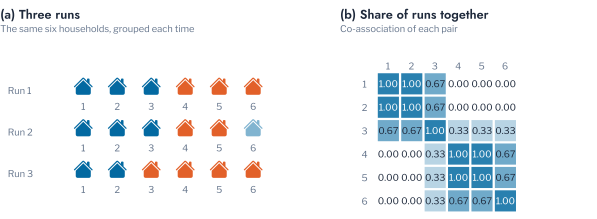
The cluster-based similarity partitioning approach of Strehl and Ghosh runs the algorithm \(r\) times on the same households and records the share of runs that place each pair together [6], [22].
\[ S_{ij} = \frac{1}{r} \sum_{m=1}^{r} \mathbb{1}\left[\lambda_m(i) = \lambda_m(j)\right]. \tag{2.13}\]
Blakely and Reno applied the same construction to the identification of the phase to which each customer is connected [23]. Over twenty runs of k-means with different starts, the mean co-association was 1.00 within the planted patterns and 0.03 across them. The measure detects sensitivity to the start of the algorithm. That sensitivity is real for k-means, because Lloyd’s algorithm converges to a local minimum (Chapter 1). It is absent here because the patterns are well separated.
Figure 2.13 shows how the matrix is built from three runs.
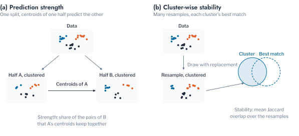
Perturbing the data tests a partition more strictly than perturbing the algorithm does. Tibshirani and Walther’s prediction strength treats clustering as an implicit classification problem [24]. The data are split into halves \(A\) and \(B\), each half is clustered into \(K\) groups, and the centroids of \(A\) predict the membership of \(B\). For each cluster \(C\) of \(B\),
\[ \text{ps}(C) = \frac{1}{n_C (n_C - 1)} \sum_{\substack{i, i' \in C \\ i \neq i'}} \mathbb{1}\left[\text{pred}(i) = \text{pred}(i')\right], \tag{2.14}\]
and the prediction strength of \(K\) is the minimum of \(\text{ps}(C)\) over the clusters of \(B\). Tibshirani and Walther recommend the largest \(K\) with a prediction strength above 0.8 to 0.9. Hennig’s cluster-wise stability judges each cluster separately [25]. The data are resampled with replacement and clustered, and each original cluster \(C\) is matched to its most similar cluster \(C'_b\) in resample \(b\).
\[ \text{stability}(C) = \frac{1}{B} \sum_{b=1}^{B} \max_{C'_b} \frac{|C \cap C'_b|}{|C \cup C'_b|}. \tag{2.15}\]
Hennig reads stability below 0.5 as dissolved, between 0.6 and 0.75 as patterned but not stable, and above 0.75 as stable. Figure 2.14 contrasts the two mechanisms.
Two variants complete the set of measures of this section. Subsample agreement clusters pairs of random subsamples and averages the ARI between the two partitions on the households that the subsamples share [26]. For \(R\) pairs of subsamples \(A_r\) and \(B_r\), with \(\lambda_{A_r}\) the labelling fitted to \(A_r\),
\[ \text{sub}(K) = \frac{1}{R} \sum_{r=1}^{R} \text{ARI}\Bigl(\lambda_{A_r}\big|_{A_r \cap B_r},\ \lambda_{B_r}\big|_{A_r \cap B_r}\Bigr). \tag{2.16}\]
The ARI of Equation 2.2 corrects the agreement of two labellings of the same households for chance. It does not correct for the reproducibility that an algorithm reaches on data without structure, which the next subsection removes. Agreement across restarts averages the ARI between partitions fitted from different single starts of the algorithm. Figure 2.15 shows the four measures for \(K\) from 2 to 7.
At \(K = 4\) the prediction strength was 0.818. About four of every five pairs of households that one half of the data groups together are grouped together again by the centroids of the other half. The least stable cluster had a stability of 0.956, which Hennig classes as stable. At \(K = 5\) the values rose to 0.900 and 1.000, because the cluster of irregular meters is as reproducible as the load patterns. At \(K = 6\) and \(K = 7\) the stability of the least stable cluster fell to 0.558 and 0.617, so one cluster of those partitions dissolves between resamples.
The two variants agree with these readings for the load patterns. Subsample agreement was 0.497 at \(K = 2\), 0.994 at \(K = 4\) and 1.000 at \(K = 5\), and agreement across restarts was 0.360, 0.930 and 1.000. The low values at two groups show that the algorithm finds no stable division of the four patterns into two halves. Stability therefore establishes that a grouping is reproducible, which is necessary, but it does not establish that the grouping is meaningful.
Calibration Against Structureless Data
A reproducibility score has no meaning until it is compared with what chance would give. The prediction strength is the share of household pairs that stay together when the clusters of one half of the data predict the grouping of the other half. For data without clusters this share is small. It also falls as the number of groups grows, because a partition of structureless data into many groups is less likely to repeat. On uniform reference data of the same size and range, the prediction strength fell from 0.510 at \(K = 2\) to 0.135 at \(K = 6\). Six groups would therefore be reproduced far less often than two even if neither division meant anything. A raw comparison across \(K\) favours small \(K\) for this reason alone.
Calibration removes this dependence on the number of groups. Let \(m(K)\) be the value of a check on the data, and \(m_0^{(r)}(K)\) its value on the \(r\)-th of \(R\) structureless reference data sets. Each reference set has the size of the data and is drawn uniformly over the range of every feature, as for the gap statistic [27]. The excess of the check over chance is
\[ \Delta_m(K) = m(K) - \frac{1}{R} \sum_{r=1}^{R} m_0^{(r)}(K), \tag{2.17}\]
and the evidence for \(K\) is its mean over the prediction strength of Equation 2.14, the stability of the least stable cluster of Equation 2.15 and the subsample agreement of Equation 2.16,
\[ \bar{\Delta}(K) = \frac{1}{3} \sum_{m} \Delta_m(K). \tag{2.18}\]
The excess measures how much of the reproducibility chance cannot explain. A value near 0 means that the partition reproduces no better than a division of structureless data. A value near 1 means that it reproduces almost perfectly where chance gives almost nothing. Figure 2.16 shows the mean excess over the three resampling checks. It was 0.181 at \(K = 2\), 0.719 at \(K = 3\) and 0.720 at \(K = 4\), and it was 0.777 at \(K = 5\) and 0.640 at \(K = 6\).
Two readings of these values follow for the load patterns. At \(K = 2\) the excess is small, so a division into two groups captures no structure of the population, and the four load patterns do not merge into two natural halves. From \(K = 3\) to \(K = 6\) the excess is large, so a partition into any of these numbers of groups reflects structure in the data and not chance. The excess does not single out four, because the load patterns and the cluster of irregular meters are both real structure. Calibration therefore answers whether a number of groups is supported by the data. It does not answer which number serves the decision, which is the question of the next section.
Pitfall: reproducible is not meaningful
A partition that survives resampling has structure, but the structure can be a small group of anomalous meters. Stability measures reproducibility and not whether the grouping serves its purpose, and a stable group too small for the decision does not serve it.
Number of Groups
The previous sections left every index and every stability measure with a failure mode. Setting the irregular meters apart raises the SC and the CHI, the inertia falls with every additional group, and stability cannot tell a load pattern from a reproducible anomaly. No single measure can therefore be trusted to choose the number of groups. This section builds the decision in four steps. A rank first combines the indices, and a check shows how much its weights matter. A minimum size taken from the decision then removes the candidates that it cannot use, and the selection rules are compared. The section ends with the cost of that minimum.
Diversity-Weighted Borda Rank
On thirty synthetic populations, the rules that read one index rarely recovered the planted four patterns. Only the DBI did so, in 10 populations. The SC, the CHI, the majority vote of the three and the inertia elbow never did.
The failures have different causes: the SC, the CHI and the majority vote chose five groups in almost every population, because setting the four irregular meters apart raises their scores. The inertia elbow never chose four, since inertia falls with every additional group and its elbow is ambiguous. The DBI is less affected by the irregular meters but is sensitive to noise. Errors with different causes need not point to the same number, which is the case for combining the indices.
A Borda count combines several indices by ranking the candidate numbers of groups on each index and summing the ranks. An index that mostly repeats others should not count as many times as an independent one, so the weights of the rank measure the independence of each index. For indices \(m = 1, \dots, M\) computed over the candidates, let \(\bar\rho_m\) be the mean absolute Spearman correlation between index \(m\) and the other indices across the candidates. The weight of index \(m\) is
\[ w_m = \frac{\max\{0.05,\ 1 - \bar\rho_m\}}{\sum_{l} \max\{0.05,\ 1 - \bar\rho_l\}}, \tag{2.19}\]
so that an index that duplicates another receives a small weight, and no index is silenced entirely. The score of a candidate \(K\) is its weighted rank sum, where \(\text{rank}_m(K)\) is the rank of \(K\) on index \(m\) after orienting every index so that larger is better.
\[ B(K) = \sum_{m=1}^{M} w_m \, \text{rank}_m(K). \tag{2.20}\]
Figure 2.17 shows the aggregation on the synthetic population: the rank of each number of groups on each index, and the weighted sum that is maximised.
The rank is made stable by three choices. The indices that improve with \(K\) by construction, the inertia and the Bayesian information criterion, are not ranked, since they would reward a large \(K\) whatever the data are. The weights are computed over every candidate, also after a constraint removes some of them, so that they do not depend on the few candidates that remain. Equal scores go to the smaller \(K\), so that the result does not depend on the order in which the candidates are listed.
Sensitivity to the Weights
The weights matter only when the indices disagree. The indices ranked are the three separation indices, the balance, the prediction strength and the stability. These six indices are the set of the book, and every later ranking uses them unchanged. The density-based and model-based indices of Section 2.2 are read beside the rank to judge a single partition and are not ranked. Figure 2.18 shows their agreement and their weights on the synthetic population. The weights are close to equal, from 0.155 for the prediction strength to 0.182 for the DBI, because no index repeats another closely. The diversity weighting therefore changes the rank little on this population.
The thirty populations show when the weights matter. At a noise level of 0.3 the diversity-weighted and equal-weight orders of the candidates agree closely, with a mean Kendall’s \(\tau\) of 0.977. The two weightings recover the four patterns in 11 and 13 populations, a difference that chance explains (\(p = 0.5\)). At a noise level of 1.0 the orders diverge, with a mean \(\tau\) of 0.767. The diversity weights then recover the four patterns in 27 populations against 16 for equal weights (\(p = 0.001\)). With a minimum size of nine the counts are 30 and 23 (\(p = 0.016\)). The advantage of the diversity weights is therefore confined to noisy data.
Figure 2.19 leaves each index out in turn and shows the change in the count. The balance and the DBI are the indices whose removal costs most. Without the balance the rank recovers four patterns in 8 populations at a noise level of 1.0, against 27 with all six indices. Without the DBI it recovers them in 1 population at 0.3, against 11. Removing the SC or the CHI, which favour five groups, raises the count at 0.3 to 19 and 20. With the minimum size every variant recovers four patterns in at least 22 populations, so no single index is necessary once the constraint is applied.
Minimum Group Size
The rank orders the candidate numbers of groups, but it cannot tell whether the best candidate serves the decision. No index in this chapter detects a small, reproducible group that cannot serve the decision. The constraint that does is not a statistical one: a group that serves a decision must be large enough for the decision. Chapter 1 announced this constraint when it tied the size of a group to what a programme can address and to what a single household reveals. A conformal threshold at a false-alarm rate \(\alpha\) needs at least
\[ n_{\min} \geq \frac{1 - \alpha}{\alpha} \tag{2.21}\]
calibration observations in each group, which is nine at \(\alpha = 0.1\) [28], [29]. Figure 2.20 shows why nine households are needed: a group of \(n\) households cannot reach a false-alarm rate below \(1/(n+1)\).
The minimum is set by the decision and not by the data. A conformal threshold at a false-alarm rate of 0.05 needs 19 households per group and one at 0.01 needs 99. A stricter guarantee therefore limits the number of groups that a few hundred households can support. A group below the minimum is removed from the candidates whatever its separation or stability.
A programme to be run on a group, a tariff to be offered to it and a network study to be based on it each impose their own minimum. The constraint is applied before the candidates are ranked, and any number of groups that produces a group smaller than the minimum is removed. It is a property of the decision and not of the data, which is why it is stated as an input and not estimated. The minimum also protects privacy, because the half-hourly profile of one household reveals when it is at home. A representative profile of few households discloses more about each of them [30].
Remark: why not estimate the minimum
A minimum size could be chosen to maximise an index, but an index cannot know what the group is for. The nine households of a conformal calibration and the households that a programme can reach come from outside the data. Estimating the minimum from the indices would reintroduce the failure that the constraint exists to remove.
Comparison of Selection Rules
The selection is the rank of the admissible candidates. A second combination weights the rank by trust. The separation score of a candidate is the weighted rank of Equation 2.20 restricted to the silhouette, the Calinski-Harabasz index and the Davies-Bouldin index, written \(B_{\text{sep}}\). It is scaled by the number of candidates \(\lvert \mathcal{K} \rvert\) to the unit interval,
\[ S(K) = \frac{B_{\text{sep}}(K)}{\lvert \mathcal{K} \rvert}. \tag{2.22}\]
The trust factor is the weaker of the balance of Equation 12.1 and the stability of the least stable cluster of Equation 2.15,
\[ T(K) = \min\Bigl\{ H(\mathbf{p}_K),\ \min_{k} \text{stability}(C_k) \Bigr\}, \tag{2.23}\]
where \(\mathbf{p}_K\) holds the group shares of the partition into \(K\) groups. The composite is their product,
\[ C(K) = S(K) \cdot T(K), \tag{2.24}\]
so that no separation can compensate for a missing trust signal. It was designed to reject a partition whose separation is high and whose reproducibility or balance is low.
Figure 7.5 counts, for each rule, the populations of thirty in which it recovered the four planted patterns. It covers noise levels of 0.3 and 1.0, with the indices alone and with a minimum size of nine. With the indices alone at the lower noise, the weighted rank recovered four patterns in 11 populations, the equal-weight count in 13 and the composite in 6. Combining the indices does not solve the problem by itself, because the group of irregular meters is reproducible and almost balanced. At five groups its balance is 0.922 and its stability 1.000, against 0.999 and 0.956 at four, and neither the composite nor the rank can reject it.
A minimum size of nine changes the outcome. At 0.3 all seven rules recover the four patterns in all thirty populations, so on clean data the constraint determines the result and the choice of index matters little. At 1.0 the weighted rank, the SC, the CHI and the composite still recover four patterns in all thirty populations. The DBI, the majority vote and the equal-weight count recover them in 23. Without the minimum the weighted rank recovers four patterns in 27 populations, against 16 for the equal-weight count and 14 for the CHI. No single index is best under every condition. The weighted rank matches or comes close to the best rule in each of the four conditions, without knowing in advance which rule that is.
Both rules read the resampling checks at their raw values, and the previous section showed that the chance level of those values falls with \(K\). A third rule uses the calibrated evidence and keeps the values of \(K\) whose excess is positive on every check,
\[ \mathcal{K}^{+} = \{\, K : \Delta_m(K) > 0 \text{ for every check } m \,\}, \tag{2.25}\]
and chooses among them the value with the largest mean excess,
\[ K^{*} = \arg\max_{K \in \mathcal{K}^{+}} \bar{\Delta}(K). \tag{2.26}\]
On the illustrative population the excess was positive on every check for \(K\) from 2 to 6. The rule alone therefore chose five groups, with a mean excess of 0.777, because the cluster of four irregular meters is as reproducible as the load patterns. A minimum size of nine removes five and six groups, and the rule then chose four groups at 0.720, narrowly ahead of three groups at 0.719. The rule ranks the values of \(K\) that the data support and cannot tell a load pattern from a small group, which only the minimum size can. Chapter 3 applies it to metered populations, where reproducibility is weaker.
The weighted rank and the calibrated excess serve different purposes, and combining them as a gate keeps the strength of each. Let \(\mathcal{K}_{\mathrm{min}}\) be the candidates that satisfy the minimum size and let \(B(K)\) be their weighted Borda rank of Equation 2.20, with the best candidate at the smallest value. The verified choice is
\[ K_{\mathrm{v}} = \arg\min_{K \in \mathcal{K}_{\mathrm{min}} \cap \mathcal{K}^{+}} B(K), \tag{2.27}\]
the best-ranked candidate whose excess is positive on every check. The gate does not reorder the candidates and therefore leaves the rank unchanged whenever its first choice passes. Ranking the excesses themselves performs worse than ranking the indices. With a minimum size of nine, the weighted rank recovered the four planted patterns in all thirty populations at noise 0.3 and 1.0. A rank of the excesses recovered them in 28 and 26 populations respectively. The excess is a noisy estimate from \(R\) reference sets, and ranking on it discards the information that the indices carry. It is used where it is reliable, as a test of whether the choice reproduces better than chance. When \(\mathcal{K}_{\mathrm{min}} \cap \mathcal{K}^{+}\) is empty, no candidate is supported by the data, and the population is reported as showing no verified grouping.
Cost of Minimum Size
The constraint removes a genuine minority pattern whenever it is smaller than the minimum. Figure 2.22 (a) shows the night pattern shrinking from 30 to 6 households in a population of 120. With the constraint the four patterns were recovered whenever the night pattern had at least nine households, and in 13% of the populations where it had six. Without it, the weighted Borda rank never recovered four patterns when the night pattern had 12 or fewer households, and did so in 43% of the populations with 30.
Figure 2.22 (b) shows that the balance responds to the same minority. At six households the balance of the partition into four groups was 0.948, below the 0.991 of the partition into three. At twelve households it was 0.971 against 0.950, and at thirty 0.999 against 0.936. The silhouette of four groups stayed between 0.681 and 0.692, above the 0.558 to 0.602 of three groups. Separation does not penalise the minority, and balance does. The indices cannot tell a small genuine pattern from a small anomalous group, and the choice cannot be left to the data. The minimum should not be lowered below what the decision needs merely to keep a minority in the partition. A minority of fewer households than the minimum is a case for inspection and not for a group. An operator who wants to keep a minority of six households has two options. The first is to lower the minimum, which the decision does not allow. The second is to treat the minority outside the partition, for example by a rule on night-time demand, which keeps the partition valid for the programmes that need the minimum.
Validation by Known Change
Internal indices, balance, stability and the choice of the number of groups all describe how well a partition is structured. None of them confirms that the partition corresponds to real behaviour. A change that is known to have happened supplies that confirmation. In the synthetic population of Chapter 1, fifteen households of the morning pattern add overnight charging of an electric vehicle at 3.7 kW from 21:00 to 01:00. If the clustering responds to behaviour, these households leave the morning pattern and form a group of their own.
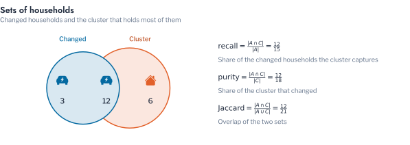
Let \(\mathcal{A}\) be the set of changed households and \(C\) the cluster that holds most of them. Three measures describe how well \(C\) recovers \(\mathcal{A}\), and each answers a different concern of an operator. The first concerns the reach of a programme addressed to the cluster. Recall is the share of the changed households that the cluster contains.
\[ \text{recall} = \frac{\lvert \mathcal{A} \cap C \rvert}{\lvert \mathcal{A} \rvert}. \tag{2.28}\]
A cluster of ten households that all changed has a recall of 0.67, because five of the fifteen changed households lie elsewhere.
The second concerns the cost of the programme. A cluster that contains every changed household can still contain many that did not change, and the offer made to the cluster is then partly wasted. Purity is the share of the cluster that changed.
\[ \text{purity} = \frac{\lvert \mathcal{A} \cap C \rvert}{\lvert C \rvert}. \tag{2.29}\]
A cluster of thirty households that contains all fifteen changed ones has a recall of 1.00 but a purity of only 0.50. The cluster of ten in the previous example reverses the pair, with a purity of 1.00 and a recall of 0.67.
Neither measure alone says whether the cluster and the changed set coincide. The Jaccard overlap does, because it divides the households that the two sets share by the households that either set contains.
\[ \text{Jaccard} = \frac{\lvert \mathcal{A} \cap C \rvert}{\lvert \mathcal{A} \cup C \rvert}. \tag{2.30}\]
It equals 1 only when the two sets are identical, and it falls whenever recall or purity falls. The cluster of ten scores 0.67 and the cluster of thirty 0.50, so a high Jaccard overlap needs a cluster that is neither too small nor diluted. Figure 2.23 shows the three measures as the overlap of two sets of households.
At five groups the recall, the purity and the Jaccard overlap were 1.00 in all thirty populations. The fifteen households fell in a single cluster that contained no other household (Figure 2.24). The partition therefore tied a group of households to a change of behaviour that its construction had not used, which no internal index can show.
On measured data the change must come from a record outside the readings. The registered photovoltaic systems of a cooperative, the tariff arms of a trial and the households to which a diversified charging profile is added each supply a set \(\mathcal{A}\). Its membership does not depend on the clustering. This is the condition under which Equation 2.28 measures validity and not the agreement of the clustering with itself.
Pitfall: an unreliable record as the reference
A record outside the readings validates a partition only if the record is reliable. Customer phase is recorded at installation and rarely corrected, so on an old network the agreement of a partition cannot exceed the share of correct records. A partition that disagrees with the record may therefore be the correct one. Audit a sample of the record first and report the agreement together with the estimated share of wrong records.
Metered Feeder
The synthetic populations have a known structure, and a metered population does not. The measures of this chapter then show whether the metered population has any structure. The population is the 342 households of a low-voltage feeder of the AusNet network, each described by its peak-normalised daily profile over 360 days. The Hopkins statistic was 0.750, against 0.501 for uniform data of the same range and 0.821 for the synthetic population. The households depart from a uniform spread, but less than the planted patterns do.
Figure 2.25 shows the indices and the resampling checks for \(K\) from 2 to 8. Every index and the weighted Borda rank chose two groups. The silhouette was 0.240 at two groups and fell to 0.144 at eight. On the synthetic population it was 0.691 at the planted four, so the groups of the feeder overlap strongly. The stability of the least stable cluster fell from 0.919 at two groups to 0.670 at four and 0.373 at eight. The prediction strength was 0.745 at two groups, below the bar of 0.8, and 0.435 at four. A partition into four or more groups of these households would not reappear on another sample of the same feeder.
The minimum size did not change the choice. The smallest group at two groups held 147 households, so minima of nine and of 34, a tenth of the households, both admit it. Partitions into six or more groups contain a group of fewer than 34 households, and the minimum of 34 removes them, but the rank had already placed them last. The selection procedure therefore returns the coarsest partition that the data support when the data hold no finer one, and the choice of rule does not matter on this feeder.
A partition that serves a tariff must also describe the households in the next period. K-means was fitted separately to the first and the second half of the year. The ARI between the two partitions of the same households was 0.412 at two groups, 0.312 at four and 0.169 at six. The agreement is well above chance but far below that of a stable grouping, and it falls as the groups become finer. The loss may come partly from the change of season between the halves and partly from the weak structure of the feeder. The readings do not separate the two causes. A tariff built on four groups would nevertheless place a large share of the households in a different group in the following period.
Validation Guide
The choice of validation depends on the decision that the partition serves. Table 2.1 sets out, for each purpose, the evidence to obtain and the minimum size of a group. The minimum also bounds the number of groups from above: \(N\) households and a minimum of \(m\) per group allow at most \(\lfloor N/m \rfloor\) groups. The 342 households of the feeder allow at most 38 groups at a minimum of nine. They allow at most three at a minimum of 100, which a tariff offer may require.
| Purpose | Evidence to obtain | Selection of the number of groups | Minimum group size |
|---|---|---|---|
| Tariff design | Clusterability; stability; external check against a tariff arm | Weighted Borda with the minimum size | Set by the smallest offer of the tariff |
| Transformer and feeder planning | Internal validity on the profile with level retained; stability | Weighted Borda with the minimum size | Set by the study, usually larger than for tariffs |
| Demand-response targeting | Recovery of a known response; purity of the target cluster | Weighted Borda with the minimum size | Set by the programme |
| Detection of irregular meters | Stability; balance; density silhouette | Weighted Borda with the minimum size | \((1 - \alpha)/\alpha\), nine at \(\alpha = 0.1\) |
| Phase or transformer identification | Agreement with verified records; stability | The number of phases or transformers is known | Not applicable |
Further Applications
The measures of this chapter apply to any partition of the objects of a distribution network. The identification of the phase of each customer, treated in Chapter 5, is the clearest case. The number of groups is known, and the records of verified customers supply an external grouping. The ARI of Equation 2.2 measures the agreement of the recovered phases with the verified ones. The co-association of Equation 2.13 measures how sensitive the recovered phases are to the start of the algorithm. The recovery of Equation 2.28 measures whether customers whose phase was changed are found. The pitfall of the previous section applies to the verified records: their share of errors bounds the agreement that any method can reach.
When the transformers and not the households are the objects grouped, the minimum size of Equation 2.21 becomes the number of transformers that a planning study needs in each class. The Hopkins statistic of Equation 2.7 then tests whether the transformers of a network form classes or are a continuum of utilisation. A distribution operator that groups feeders by loading and finds a Hopkins statistic near 0.5 should plan for the continuum and not for classes. The same sequence applies to the photovoltaic systems of Chapter 1. The Hopkins statistic tests whether the arrays form classes by orientation. A stable group of few arrays is checked against the minimum size before it is treated as a class.
A third use is the persistence of a partition over time, which the feeder of the earlier section illustrated. The ARI of Equation 2.2 between partitions fitted to two periods validates a partition without labels, and the finer partitions persisted least.
Conclusion
This chapter defined the measures that judge a partition and the rules that select the number of groups. Agreement with a known grouping is scored by the adjusted Rand index. It is corrected for chance, so it is the only one of the three measures that can compare partitions with different numbers of groups. The Hopkins statistic tests first whether the data contain groups, and the connectivity of the neighbourhood graph tests whether they stand apart. Internal indices measure compactness and separation, and each fails on a case from the low-voltage grid. The separation indices prefer an isolated pair of irregular meters, and the SC prefers a partition that crosses crescents. A density-based index resists both failures but costs more to compute. Balance detects the first failure and is itself lowered by a genuine minority. Stability showed that a grouping is reproducible and did not show that it is meaningful, and calibration against structureless data showed which numbers of groups the data support.
Selecting the number of groups from one index chose five groups, since the cluster of four irregular meters scores well on the separation indices and is reproducible. The diversity-weighted Borda rank combines the indices and weights each by its independence. Clean data showed no effect of the weights. At a noise level of 1.0 they raised the recovery of the planted number from 16 populations of thirty to 27 (\(p = 0.001\)). The constraint that determines the outcome is a minimum group size taken from the decision that the groups serve. With it, every rule recovered the planted number in all thirty populations on clean data. At the higher noise level the diversity-weighted rank kept that result, and the DBI and the equal-weight count did not. The constraint removes a genuine minority smaller than the minimum, which is its cost. A final check verifies the choice against chance. The best-ranked candidate must also exceed structureless data on every resampling check (Equation 2.27), so a rank is a proposal and the verified value is the result. A rank of the excesses themselves recovered the planted number in 28 and 26 populations of thirty at the two noise levels, against 30 for the weighted rank. External validation against a known change of behaviour, here overnight charging, tied a cluster to behaviour with a recall, purity and Jaccard overlap of 1.00.
Chapter 3 applies the same measures to metered data from three utilities, where none of the structure is known in advance. The chapter does not establish that the partitions it selects serve a particular tariff or network study. That requires the outcomes of the decision, which Chapters 4 to 6 of this part examine.
Remark: scope and limitations
These conclusions rest on the synthetic populations of Chapter 1, whose structure is known and that are free of anomalies apart from the meters added to them. The selection was repeated on thirty populations and applied to one metered feeder. On the feeder, where the structure is weak, every rule chose two groups, and the minimum size did not bind.
The scope of these conclusions is the synthetic population and one metered feeder, and Chapter 3 extends them to three populations.
Key findings
The adjusted Rand index is the only one of three measures of agreement that does not reward more groups. Separation indices preferred a partition that isolates two irregular meters, and balance alone detected it. Resampling showed the isolated group to be as reproducible as the load patterns. A minimum group size taken from the decision enabled every rule to recover the planted number. It was nine households for a conformal threshold at a false-alarm rate of 0.1. It also removed a genuine minority smaller than the minimum. The diversity weights of the Borda rank helped only on noisy data. A known change of behaviour was recovered with a recall, purity and Jaccard overlap of 1.00. A density-based index was the only single index to choose the planted number independently of group sizes. On a metered feeder every rule chose two groups, which the weak structure of the feeder supports.
Exercises
- Show that the adjusted Rand index of Equation 2.2 has expectation zero when the two partitions are drawn independently with fixed group sizes. Explain why the purity of Equation 2.6 does not.
- Derive the minimum number of calibration observations \((1 - \alpha)/\alpha\) of Equation 2.21. Use the requirement that the empirical quantile of \(n\) calibration scores at level \(1 - \alpha\) exists. State the minimum for \(\alpha = 0.05\).
- Show that two indices with identical rankings across the candidates receive together the weight of one independent index in Equation 2.19, up to the floor of 0.05.
- A population of \(N\) households and a minimum group size \(m\) allow at most \(\lfloor N/m \rfloor\) groups. Show why, and find the candidate numbers of groups that remain for a feeder of 342 households at minima of nine, 34 and 100.
- Explain why the balance of Equation 12.1 falls when a partition recovers a genuine minority pattern. State one use of balance for which this fall is a correct signal and one for which it is not.
- A utility has 60,000 smart-meter profiles and wants to fix a tariff for three groups of customers, with no topology records and no labels. Choose the partition, state the evidence to obtain before and after clustering, and justify the minimum group size.