Foundations of Retrieval, Ranking and Recommendation
A Distribution System Operator (DSO) answers questions about individual customers and transformers every day, and most of them have the same form. A request to connect rooftop Photovoltaic (PV) arrives, and the operator must judge whether the network can host it, usually before any study has been run. The transformers of a network must be examined in some order, because the capacity to examine all of them at once does not exist. A transformer that violates its limits needs a remedy, and several are available, from settings on the customers’ inverters to a larger transformer. Part 5 showed that groups of customers answer none of these questions well. Archetypes of the shape of demand accounted for 5.3% of the variance of a customer’s contribution to the transformer peak, while three quarters of the variance of the worst voltage lay between customers of the same transformer. The answer has to be given for the individual case.
Questions about individual cases are not new to machine learning. Information retrieval finds the items most relevant to a query and orders them [1]. Recommender systems choose items for users of whom little may be known [2], [3]. Case-based reasoning solves a new problem by reusing the solution of a similar one [4], and causal inference asks what an action changes rather than what accompanies it [5], [6]. Each field supplies a formal statement of one step of a decision and a way to evaluate it. None was designed for a distribution network, however, and none assumes what this part can assume, namely a simulator that returns the outcome of every action for every case.
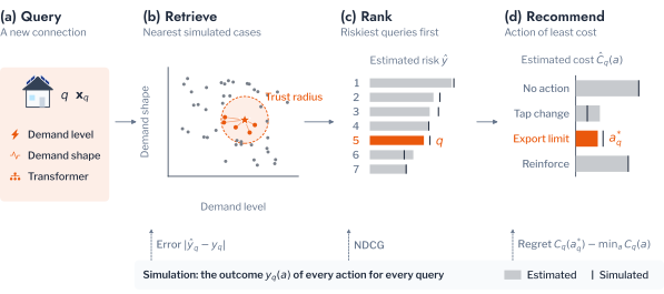
This chapter brings the four fields together for the Low Voltage (LV) network. It frames the decisions of a DSO as a chain of retrieval, ranking and recommendation (Figure 6.1), in which each step consumes the output of the one before. Retrieval estimates the outcome of a new case from similar ones, and raises the question of when such an estimate can be trusted. Ranking orders the cases by their estimated outcome, and raises the question of how an order is judged and learned. Recommendation assigns each case a mitigation measure, and raises the question of how the effect and the cost of a mitigation measure are estimated from records in which each transformer received only one. The chapter reviews the literature on each step, states the steps in one notation, and answers the three questions in turn on a synthetic case base whose outcome under every mitigation measure is known. Chapter 2 then applies retrieval to the AusNet networks, Chapter 3 applies ranking, and Chapter 4 applies recommendation.
Retrieval, Ranking and Recommendation in the Literature
The review follows the chain of Figure 6.1, from the retrieval of similar cases to the choice of an action, and closes with the work that has applied these ideas to energy networks.
Retrieval in its simplest form answers a query with the items nearest to it under a measure of similarity. The nearest-neighbour rule of Cover and Hart is its statistical foundation: as the number of stored cases grows, the error of the rule approaches a small multiple of the least achievable error [7]. A retrieval returns several items, and information retrieval therefore evaluates the answer as a ranked list, crediting relevant items more the nearer they are placed to the top [1]. Järvelin and Kekäläinen extended this credit to graded relevance through the discounted cumulative gain [8], now the standard measure of a ranked list.
Once a list is judged by its order, the order itself can be learned. Learning to rank fits a score whose order matches the relevance of the items, rather than the relevance of each item, and Liu classified its methods as pointwise, pairwise and listwise, according to whether the loss is computed on single items, on pairs or on whole lists [9]. RankNet introduced the pairwise logistic loss on the difference of two scores [10]. LambdaRank then weighted the gradient of each pair by the change in a listwise measure that swapping the pair would cause [11], and LambdaMART fitted these gradients with gradient-boosted trees [12], [13]. Chen and colleagues later showed that the pairwise losses of these rankers bound one minus the NDCG of the list, so that minimising them improves the measure by which a list is judged [14].
Recommender systems extend ranking from the items relevant to a query to the items suited to a user. They are commonly divided into content-based methods, which recommend from the features of an item, collaborative methods, which recommend from the behaviour of similar users, and hybrids of the two [2], [15], [16]. Matrix factorisation, the dominant collaborative method, learns latent factors from a large and sparse matrix of interactions [17], and a user or item without history therefore defeats it, a difficulty known as the cold start [18]. Recommendations are usually evaluated offline on logs of past interactions, by the accuracy of predicted ratings and of ranked lists [19], [20]. A log, however, records only the response to items that were shown, and unbiased offline evaluation reweights it by the probability with which each item was shown [21], [22].
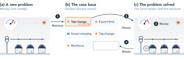
The limitation of the log is a causal one, and it is shared by the oldest method of recommending a remedy. Case-based reasoning, as formalised by Aamodt and Plaza, solves a problem in a cycle of four steps: retrieve the most similar past case, reuse its solution, revise the solution by testing it, and retain the solved case [4]. The cycle assumes that the retained cases record what each solution achieved. Causal inference states what such a record can and cannot reveal. Rubin defined the effect of a treatment through its potential outcomes, of which only one can be observed for each unit [5], and Holland called this the fundamental problem of causal inference [23]. Rosenbaum and Rubin stated the conditions under which an effect can nevertheless be estimated from observational records [24], and Künzel, Sekhon, Bickel and Yu combined ordinary regressors into estimators of the effect on each unit, the meta-learners [25].
Two concerns cut across all three steps, the reliability of an estimate and the fairness of a list. Conformal prediction addresses the first: it turns any score into a set or an interval with a guaranteed coverage under exchangeability, without assumptions on the model [26], [27], [28], [29]. It was used for cluster membership in Part 5, Chapter 3 (Equation 3.19), and for intervals on electricity prices by Kath and Ziel [30]. Fairness of exposure addresses the second, by constraining how the attention of a ranked list, which falls with position, is shared among groups [31]; maximal marginal relevance similarly trades relevance against redundancy within a list [32].
In the energy domain these ideas have been applied separately. Qammar and colleagues estimated hosting capacity by clustering [33], Andagoya-Alba and colleagues estimated it without a network model [34], and Duran and Monti recommended where PV should be adopted [35]. Luo and colleagues built a recommender on disaggregated loads [36], Gangwar and Shaik used nearest neighbours for protection [37], and Parvez, Hu and Chen ranked floods of similar alarms for operators [38]. Each work addresses one step, and none evaluates against the outcome of every action. Assembling the steps into one chain first requires a common statement of the problem, which the next section provides.
Problem Formulation and Notation
The decisions of this part share one structure. A query \(q\), which may be a connection request, a customer, a transformer or a violation event, is described by a vector of features \(\mathbf{x}_q\). A case base \(\mathcal{D} = \{(\mathbf{x}_j, y_j)\}\) holds cases whose outcomes are known, and a set \(\mathcal{A}\) holds the actions available, including no action, written \(a = 0\). The potential outcome \(Y_q(a)\) is the outcome of query \(q\) had action \(a\) been taken. In this chapter it is the number of hours the voltage spends outside the statutory band. Each action also has a cost \(C_q(a)\), defined in Equation 6.27.
In this notation the three steps of the chain differ only in what they produce. Retrieval produces an estimate \(\hat y_q\) of the outcome of a new query from the cases nearest to it. Ranking produces an order of a set of queries from a score such as \(\hat y_q\). Recommendation produces for each query the action of least estimated cost,
\[ \hat a_q = \arg\min_{a \in \mathcal{A}} \hat C_q(a). \tag{6.1}\]
The three outputs are evaluated against different quantities, and here the simulator becomes essential. The field observes only \(Y_q(\hat a_q)\), the outcome of the action taken. The simulator observes \(Y_q(a)\) for every \(a\), so that each step can be scored exactly. Retrieval is scored by its error, ranking by the order of the true outcomes, and recommendation by the cost it forgoes. Table 6.1 maps the vocabulary of retrieval and recommendation onto the network, and Table 6.2 collects the notation, which extends that of Part 5 (Table 1.1).
| Concept | Retrieval and recommender systems | Low-voltage network |
|---|---|---|
| Query | A search or a user | A connection request, transformer or violation event |
| Case or item | A document or a product | A simulated transformer with known outcomes |
| Relevance | A graded judgement or a rating | Hours outside the statutory band |
| Action | An item shown to a user | A mitigation measure applied to a transformer |
| Feedback | Responses to the items shown | The field record of the mitigation measure applied |
| Counterfactual | Responses to items not shown | Simulated outcomes of the other mitigation measures |
| Cold start | A user or item without history | A connection without a network study |
| Symbol | Description |
|---|---|
| \(q\), \(\mathbf{x}_q\) | Query and its features |
| \(\mathcal{D}_1\), \(\mathcal{D}_2\) | Cases kept for retrieval, and \(n\) held-out calibration cases |
| \(\mathcal{A}\), \(a\) | Set of actions (mitigation measures) and one action; \(a = 0\) is no action |
| \(Y_q(a)\) | Potential outcome of \(q\) under \(a\), in hours outside the band |
| \(\tau_q(a)\) | Uplift of \(a\), the hours it removes relative to no action |
| \(C_q(a)\), \(\mathrm{Reg}_q\) | Total cost of \(a\) for \(q\), and regret of a recommendation |
| \(\mathcal{N}_k(q)\), \(\hat y_q\) | The \(k\) kept cases nearest to \(q\), and the estimated outcome |
| \(s(\mathbf{x})\), \(\hat r\) | Distance to the nearest kept case, and trust radius |
| \(\gamma_i\), \(\varepsilon\) | Residual score of a held-out case, and its conformal quantile |
| \(\hat\sigma(\mathbf{x})\), \(z_q\) | Local scale of the residuals, and group of a query |
| \(m\), \(K\) | Number of items in a list or of units sharing a burden, and cut-off of a list |
| \(\mathrm{rel}_i\), \(w_i\), \(f_i\) | Relevance grade, weight and score of the item in position \(i\) |
| \(\rho_a(\mathbf{x})\), \(\omega\) | Propensity of action \(a\), and share of treated cases |
| \(\pi\), \(V(\pi)\) | Policy, and its mean cost |
| \(G(\mathbf{b})\) | Gini coefficient of a burden \(\mathbf{b}\) |
An Illustrative Case Base
Scoring every step exactly requires a population in which \(Y_q(a)\) is known for every mitigation measure, and a synthetic case base supplies one before the AusNet networks of Chapter 2. It contains 600 transformers on four networks. Transformer \(i\) serves a feeder of electrical length \(L_i\), with a share \(p_i\) of customers with rooftop PV, a share \(e_i\) charging an Electric Vehicle (EV) in the evening, and a level of demand \(d_i\). Its voltage at the end of the feeder over a clear day is
\[ v_i(t) = v_0 + L_i \bigl( \kappa_i p_i\, g(t) - \beta_d d_i\, u(t) - \beta_e e_i\, c(t) \bigr), \tag{6.2}\]
where \(v_0 = 1.03\) pu is the sending voltage, \(g\), \(u\) and \(c\) are the profiles of PV output, household demand and evening charging, \(\beta_d\) and \(\beta_e\) are sensitivities, and \(\kappa_i\) is the strength of the PV voltage rise, which varies between transformers and is not among the features. The four networks differ in the length of their feeders, from urban to rural.
The inverters of every case respond to voltage as AS/NZS 4777.2 requires of them, which no operator chooses. Their volt-watt response leaves PV output unrestricted up to 253 V (1.10 pu) and curtails it to 20% at 260 V, so it holds the voltage near the upper limit rather than inside the band; their volt-VAr response lies outside a model without reactive power. The mitigation measures of the network operator are stated as changes to the terms of Equation 6.2. Smart charging moves the charging term to the night, an export limit caps PV export at 70% of its peak, a tap change lowers the transformer’s off-load tap one step and with it \(v_0\) by 2.5%, and reinforcement with a larger transformer removes 40% of every voltage change. The outcome \(Y_i(a)\) is the number of hours \(v_i\) spends outside the AS 61000.3.100 band of 0.94 to 1.10 pu under mitigation measure \(a\).
Without action, 60.8% of the transformers left the band at some hour, 35.8% rising above it at midday and 47.5% falling below it in the evening (Table 6.3). Reinforcement reduced the mean hours outside the band from 2.72 to 0.45, while the tap change raised them to 3.02, because the evening hours it adds outweigh, on average, the midday hours it removes. No mitigation measure was the cheapest everywhere. Under the costs of Equation 6.27, no action was the cheapest for 41.3% of the transformers, reinforcement for 26.0%, smart charging for 19.8% and the tap change for 3.8%, those whose only violation is at midday. The choice of mitigation measure is therefore a decision for each transformer, and the case base is a fair test of the methods that make it.
The case base is split at random into 300 transformers kept for retrieval, 150 held out for calibration and 150 for testing. The four features \(L\), \(p\), \(e\) and \(d\) are standardised on the kept transformers. The kept transformers play the role of the studies a utility has already run, and the test transformers the role of new requests, which is where the chain begins.
Retrieval Under a Trust Radius
A new connection request is the first decision of the chain, and it usually arrives without a network study. This section estimates its outcome from the case base, and then asks when that estimate deserves to be used.
Nearest Neighbours and the Trust Radius
A request without a study is a cold start in the sense of recommender systems. The query has no outcome of its own, and with no history of interactions its outcome can only be estimated from the content of similar cases. The estimate of this part is the mean outcome of the \(k\) nearest kept cases,
\[ \hat y_q = \frac{1}{k} \sum_{j \in \mathcal{N}_k(q)} y_j, \tag{6.3}\]
with \(k = 10\) and the Euclidean distance on the standardised features. Equation 6.3 returns an estimate for every query, including one unlike any case in \(\mathcal{D}_1\), whose nearest neighbours describe it poorly. A request from a household unlike any simulated, or from a network with longer feeders, is such a query. The estimate therefore needs a rule that decides when to answer from the case base and when to run a study instead, and the trust radius of Figure 6.2 is that rule.
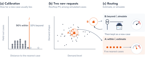
The radius has to refuse few queries that resemble the case base, and conformal prediction sets it with that guarantee. It follows the split-conformal construction of Part 5, Chapter 3 (Equation 3.19), with the distance to the case base as the nonconformity score [26], [27]. The score of a query is its distance to the nearest kept case,
\[ s(\mathbf{x}) = \min_{j \in \mathcal{D}_1} \lVert \mathbf{x} - \mathbf{x}_j \rVert. \tag{6.4}\]
The held-out cases calibrate this score. Let \(s_{(1)} \le \dots \le s_{(n)}\) be the ordered scores of the \(n\) cases of \(\mathcal{D}_2\). The trust radius at level \(\alpha\) is the order statistic
\[ \hat r = s_{(\lceil (n + 1)(1 - \alpha) \rceil)}. \tag{6.5}\]
If a query is exchangeable with the held-out cases, it lies within the radius with probability
\[ 1 - \alpha \le \Pr\{ s(\mathbf{x}_q) \le \hat r \} \le 1 - \alpha + \frac{1}{n + 1}, \tag{6.6}\]
the upper bound holding when the scores have no ties [28], [29]. At most a share \(\alpha\) of the queries that resemble the case base is therefore refused. The converse is also informative, since a refusal rate well above \(\alpha\) on a new population measures how far that population has shifted. The same test can be written with the conformal p-value
\[ p(\mathbf{x}_q) = \frac{1 + \#\{ i \in \mathcal{D}_2 : s_i \ge s(\mathbf{x}_q) \}}{n + 1}, \tag{6.7}\]
with refusal when \(p(\mathbf{x}_q) \le \alpha\) [26].
Error Intervals
The radius guarantees that a trusted query is close to some case, but closeness does not make its estimate accurate. A second calibration, on the outcomes rather than the features, supplies an interval with its own guarantee. The residual score of a held-out case is
\[ \gamma_i = \frac{|y_i - \hat y_i|}{\hat\sigma(\mathbf{x}_i)}, \tag{6.8}\]
and \(\varepsilon\) is its order statistic by the rule of Equation 6.5. The interval
\[ \mathcal{C}(\mathbf{x}_q) = \bigl[ \hat y_q - \varepsilon\, \hat\sigma(\mathbf{x}_q),\ \hat y_q + \varepsilon\, \hat\sigma(\mathbf{x}_q) \bigr] \tag{6.9}\]
then covers a new outcome with probability at least \(1 - \alpha\). The scale \(\hat\sigma\) determines the shape of the interval. With \(\hat\sigma \equiv 1\) the interval has a fixed width. With \(\hat\sigma = \hat\sigma_k\), the standard deviation of the outcomes of the \(k\) nearest cases, it is the locally weighted interval of Lei and colleagues [28], wider where the neighbours disagree (Figure 6.3).
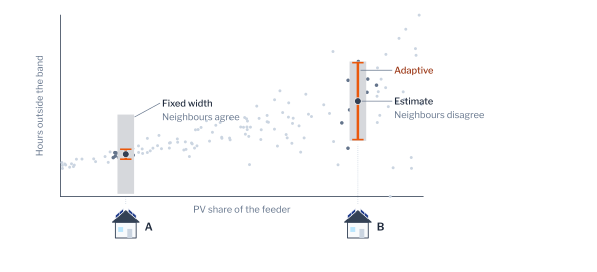
Both guarantees hold on average over all queries, whereas a utility may need them within each part of its network. Both calibrations can therefore be made separately for each group \(z\) of cases, such as a network or a violation pattern, and the guarantee then holds within each group,
\[ \Pr\{ Y_q \in \mathcal{C}(\mathbf{x}_q) \mid z_q = z \} \ge 1 - \alpha, \tag{6.10}\]
rather than only on average over the groups [26].
The guarantee within groups has a price in data. A conformal quantile at level \(1 - \alpha\) requires at least \((1 - \alpha)/\alpha\) calibration cases in each group, nine at \(\alpha = 0.1\), and the interval widens as the number of cases in a group falls, so a utility that calibrates by network or by violation pattern must hold back enough simulated cases for each. The width of the interval is itself the useful output for a planner. A narrow interval on the safe side of a limit supports a decision without a study, and an interval that contains the limit identifies a connection that a study must resolve, which is the decision rule that Chapter 2 builds on this interval.
Retrieval on the Case Base
The estimate, the radius and the interval were applied to the test transformers, and to a second population drawn to differ from the case base. Retrieval reduced the mean absolute error from 2.61 hours, that of the mean of the kept cases, to 1.17 hours for the queries it trusted (Table 6.4). The radius, calibrated at \(\alpha = 0.1\), trusted 87.3% of the test transformers. Queries from a population whose feeders were drawn between 1.0 and 1.8 rather than between 0.5 and 1.2, before the factor of each network, were trusted in only 51.3% of cases. Those refused were estimated with an error of 2.04 hours against 1.53 hours for those trusted, so the radius both detected the shift and identified the queries it affected most.
The interval appeared less reliable on this split. The adaptive interval covered 84.7% of the trusted test outcomes, below the nominal 90%. The guarantee of Equation 6.6, however, is an average over random splits, and a single split of 150 test cases varies around it by several points. Over 200 random splits the trust radius admitted 89.9% of the test transformers, the fixed-width interval covered 90.1% and the adaptive interval 89.9%, against a finite-sample floor of 90.07% (Table 6.5). The adaptive interval reached this coverage with a mean width of 4.41 hours against 5.82 hours for the fixed width, 24% narrower, because it concentrated its width on the queries whose neighbours disagreed. For a utility, a narrower interval with the same guarantee means that fewer connection requests have an interval that contains the limit, and so fewer are referred for a study.
Figure 6.4 shows the 200 splits behind these means. The coverage of a single split ranged from below 80% to above 95%, with a standard deviation of 3.3 percentage points for the adaptive interval, so a utility that checks the guarantee on one split may conclude that it fails when it holds. The guarantee of Equation 6.6 is a property of the procedure over exchangeable splits, not of one split, and it is verified over repeated splits or, in operation, over successive periods, as Part 7 does for the false-alarm rate of a detector.
A conformal guarantee is a property of the procedure, averaged over the random choice of the calibration and test cases, and a single evaluation can fall below it by chance. A coverage reported for one split should be read with its sampling variation, here a standard deviation of about 3 points. A claim that a method under-covers requires repeated splits.
A trusted estimate with a calibrated interval answers a single request. A utility, however, holds many transformers at once and can study only some of them, so the estimates must next be compared across transformers.
Ranking and Its Evaluation
Comparing transformers turns retrieval into ranking, and the quality of a ranking depends on where its errors fall. This section first defines how an order is judged, then how it can be learned, and then compares both on the case base.
Measures of a Ranked List
A DSO that examines transformers in order of estimated risk needs the order to be correct at the top, where the examinations happen. Let a score place the \(m\) transformers of one list in positions \(i = 1, \dots, m\), and let \(\mathrm{rel}_i \ge 0\) be the relevance grade of the item in position \(i\). Here the grade is the hours outside the band; Figure 6.5 uses four illustrative levels instead. The simplest measures look only at the first \(K\) positions. With \(S_K\) the items in those positions and \(T_K\) the \(K\) most relevant items, precision at \(K\) is
\[ \mathrm{P}_K = \frac{|S_K \cap T_K|}{K}. \tag{6.11}\]
The reciprocal rank looks only at the most relevant item, placed at position \(i^\star\),
\[ \mathrm{RR} = \frac{1}{i^\star}, \tag{6.12}\]
and its mean over the lists is the mean reciprocal rank, Mean Reciprocal Rank (MRR). Precision counts an item as relevant or not, and the reciprocal rank follows a single item, so neither distinguishes a near miss from a gross error. The discounted cumulative gain does, by weighting the grade of each position [8],
\[ \mathrm{DCG}_K = \sum_{i=1}^{K} \mathrm{rel}_i\, w_i, \tag{6.13}\]
with the weight of position \(i\) decreasing logarithmically,
\[ w_i = \frac{1}{\log_2(i + 1)}. \tag{6.14}\]
The gain is linear in the grade. The exponential gain \(2^{\mathrm{rel}_i} - 1\), common in web search [11], is appropriate for grades on a short ordinal scale and would make hours outside the band meaningless as a gain. Because \(\mathrm{DCG}_K\) grows with the grades of the list, lists are compared after dividing by the gain of the ideal order, \(\mathrm{IDCG}_K\),
\[ \mathrm{NDCG}_K = \frac{\mathrm{DCG}_K}{\mathrm{IDCG}_K}, \tag{6.15}\]
which equals one for a perfect ranking (Figure 6.5).
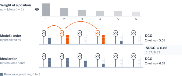
The top of the list is not the only concern of a planner, who may study the remaining transformers in order as well. Kendall’s coefficient measures the agreement of two orders over the whole list [39]. Many transformers of a list share the same grade, since 39% have no hours outside the band, and the coefficient is therefore taken in its form corrected for ties,
\[ \tau_{\mathrm{b}} = \frac{\nu_{\mathrm{c}} - \nu_{\mathrm{d}}}{\sqrt{(\nu_0 - \nu_{\mathrm{rel}})(\nu_0 - \nu_f)}}, \tag{6.16}\]
where \(\nu_{\mathrm{c}}\) and \(\nu_{\mathrm{d}}\) count the concordant and discordant pairs, \(\nu_0 = m(m - 1)/2\) is the number of pairs, and \(\nu_{\mathrm{rel}}\) and \(\nu_f\) count the pairs tied in grade and in score. With one list per network, each measure is averaged over the four networks.
Learning to Rank
The measures judge a score, and the next question is where the score comes from. It can be the estimate of Equation 6.3, which is fitted to the outcome of each transformer and ranks only as a consequence. A pointwise loss of this kind fits each grade separately, as a regression does,
\[ \ell_i = (f_i - \mathrm{rel}_i)^2, \tag{6.17}\]
where \(f_i\) is the score of item \(i\). The score can instead be learned to order the list directly. A pairwise loss penalises each pair with \(\mathrm{rel}_i > \mathrm{rel}_j\) that the scores order wrongly, through the logistic loss of RankNet [10],
\[ \ell_{ij} = \log\bigl(1 + e^{-(f_i - f_j)}\bigr). \tag{6.18}\]
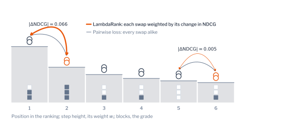
The pairwise loss counts every misordered pair equally, whereas Equation 6.15 weights errors by position. LambdaRank closes this gap by weighting the gradient of each pair by the change in Normalised Discounted Cumulative Gain (NDCG) that swapping the two items would cause [11],
\[ \lambda_{ij} = -\frac{|\Delta \mathrm{NDCG}_{ij}|}{1 + e^{f_i - f_j}}, \tag{6.19}\]
so that errors near the top of a list cost most (Figure 6.6). The loss remains pairwise, but its weights come from a listwise measure, which places LambdaRank between the pairwise and listwise families of Liu [9]. LambdaMART fits these gradients with boosted regression trees [12]. The ranker of this part grades the outcome of each list into five quantile levels and fits LambdaMART on them.
The choice between the families depends on how the ranking will be used. When the score is accurate, a pointwise estimate orders the list well, since a ranking can be wrong only where two estimates are wrong by more than the gap between their outcomes. When a utility acts only on the first few transformers of a long list, as a programme of inspection does, the errors that matter are those near the top, and the position weights of Equation 6.19 concentrate the fit there. The comparison on the case base and on the networks of Chapter 3 tests whether this advantage survives the small lists of a distribution network.
Ranking on the Case Base
The two sources of a score, the pointwise estimate and the learned ranker, were compared with two baselines on the test transformers of each network. A single split of the case base varies too much to separate them, so the comparison was repeated over the 200 random splits used for coverage, and each pair of scores was compared split by split with a Wilcoxon signed-rank test. The nearest kept cases ranked best on every measure, with an NDCG at 10 of 0.858 and \(\tau_{\mathrm{b}}\) of 0.633, against 0.841 and 0.588 for LambdaMART (Table 6.6). The advantage in NDCG was small, 0.016 on average and present in 71% of the splits, but significant (\(p < 10^{-9}\)). The advantage in \(\tau_{\mathrm{b}}\) was larger and more consistent, present in 93% of the splits (\(p < 10^{-30}\)), so the estimate ordered the whole list better than the ranker trained to order it. The MRR differed least, 0.533 against 0.500, with the nearest cases ahead in 59% of the splits (\(p = 0.008\)).
Ranking by the PV share alone, a heuristic available to any utility, reached an NDCG of 0.649 and an MRR of 0.317, and a random order 0.368 and 0.105. The PV share therefore captured part of the risk but ordered neither the top nor the rest of the list as well as the case base, since the evening under-voltage of a transformer depends on its charging and demand rather than its PV. With 300 kept transformers and four features, a ranker learned for the purpose did not improve on the estimate it ranks. Whether learning to rank helps on larger and more varied lists is examined in Chapter 3.
A ranked list tells a utility where to act but not what to do. The last step of the chain chooses the mitigation measure, and it requires a different kind of estimate.
Recommendation as a Causal Question
Retrieval and ranking estimate the outcome of a transformer as it is. Recommendation must estimate how the outcome would change under each mitigation measure, which is a causal question. This section starts from the practice of reusing past remedies, shows why field records bias it, states the estimators that correct the bias, and then judges recommendations by their cost.
Utilities already recommend remedies from experience, and case-based reasoning formalises that practice (Figure 6.7). A planner retrieves the transformer most like the new one, reuses its remedy, revises the remedy if a study shows that it fails, and retains the solved case. The cycle is sound when the cases record what each remedy did. A field record, however, holds one outcome per transformer, that of the action taken, and the next subsection states what this omission costs.
Potential Outcomes and Confounding
What a remedy did is a comparison between two potential outcomes. The effect of action \(a\) on query \(q\) is its uplift, the hours it removes relative to no action,
\[ \tau_q(a) = Y_q(0) - Y_q(a). \tag{6.20}\]
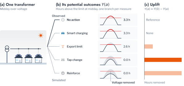
Only one of the two potential outcomes is observed in the field (Figure 6.8). An estimate from a field record must therefore compare different transformers, those that received the action, \(A = a\), and those that did not. The naive comparison of their means decomposes as
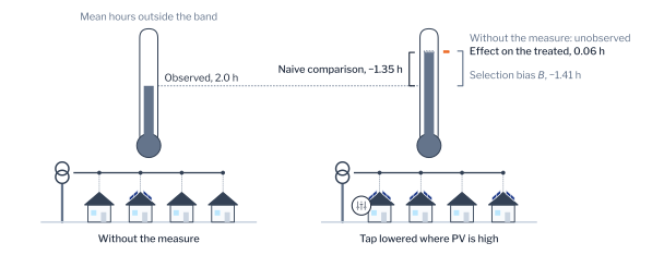
\[ \mathbb{E}[Y \mid A = 0] - \mathbb{E}[Y \mid A = a] = \tau_{\mathrm{T}} + B, \tag{6.21}\]
where \(\tau_{\mathrm{T}} = \mathbb{E}[\tau(a) \mid A = a]\) is the effect on the treated transformers and
\[ B = \mathbb{E}[Y(0) \mid A = 0] - \mathbb{E}[Y(0) \mid A = a] \tag{6.22}\]
is the selection bias [6]. A utility applies a mitigation measure where the problem is worst, so the treated transformers have the larger \(Y(0)\), \(B\) is negative, and the naive comparison understates the effect (Figure 6.9), in the case base enough to make a mitigation measure that changes little appear harmful.
The bias arises because the choice of action depends on the transformer, and it can be removed when that dependence is captured by the features. The effect can then be estimated from observational records under two conditions [24]. The first is that every feature that influenced the choice of action is among the features,
\[ \{ Y(0), Y(a) \} \perp\!\!\!\perp A \mid \mathbf{x}. \tag{6.23}\]
The second is that every transformer could have received either action, with propensity
\[ 0 < \rho_a(\mathbf{x}) = \Pr\{ A = a \mid \mathbf{x} \} < 1. \tag{6.24}\]
Neither condition can be verified from the record itself, and a utility must argue the first from how its decisions were made. A randomised assignment satisfies both by construction, since the action then depends on no feature and every unit has the same propensity. The time-of-use arm of the Low Carbon London trial, to which households were assigned at random, is such a record, and the further applications of this chapter use it to estimate how the response to a price varies between households.
Meta-Learners
Under these conditions the effect can be estimated by comparing transformers with the same features, and the meta-learners of Künzel and colleagues do so with ordinary regressors [25]. The T-learner fits a model \(\hat\mu_0\) of the outcome on the untreated cases and a model \(\hat\mu_1\) on the treated cases, and estimates
\[ \hat\tau(\mathbf{x}) = \hat\mu_0(\mathbf{x}) - \hat\mu_1(\mathbf{x}), \tag{6.25}\]
with the sign of Equation 6.20. When one group is small, its model is poor and so is the difference. The X-learner reduces this dependence by imputing an effect for each case from the model of the other group, \(\tilde\tau_i = \hat\mu_0(\mathbf{x}_i) - y_i\) for a treated case and \(\tilde\tau_i = y_i - \hat\mu_1(\mathbf{x}_i)\) for an untreated one. It regresses the imputed effects on the features within each group, giving \(\hat\tau_1\) and \(\hat\tau_0\), and combines them with the share \(\omega\) of treated cases,
\[ \hat\tau(\mathbf{x}) = \omega\, \hat\tau_0(\mathbf{x}) + (1 - \omega)\, \hat\tau_1(\mathbf{x}), \tag{6.26}\]
so that the regression built on the model of the larger group receives the larger weight (Figure 6.10).
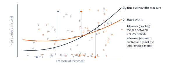
To test the estimators against a known effect, a field record was generated in which the tap was lowered with a probability that rose with the PV share, reaching 49.1% of the kept and held-out transformers. The effect of the tap change differs in sign between transformers, removing midday hours where PV dominates and adding evening hours where charging does, and its simulated uplift on the test transformers averaged \(-0.29\) hours. The naive comparison estimated \(-1.26\) hours, four times the harm, because the treated transformers were those with the most PV and the worst baseline, as Equation 6.22 predicts (Table 6.7). The T-learner estimated \(-0.35\) hours and the X-learner \(-0.29\) hours. For individual transformers the X-learner was the more accurate, with an error of 1.44 hours against 1.69 hours and a correlation with the simulated effect of 0.48 against 0.45. The X-learner is therefore the better choice where the effect on each transformer, rather than the average, informs the decision, and where one action is rare in the record, as the cross-imputation of Equation 6.26 borrows from the larger group.
Figure 6.11 places the three estimates against the simulated effect. The naive comparison lay 0.98 hours from it, the T-learner 0.06 hours and the X-learner within 0.01 hours. The field record of a utility is confounded in the same way, since a mitigation measure is applied where the problems are worst, and the comparison of treated and untreated transformers in that record attributes the difference between them to the measure. An estimate of the effect of a measure from operational records is therefore credible only when it conditions on the features that drove the choice of the measure, the condition of Equation 6.23, and the meta-learners are the means of doing so.
Cost and Regret
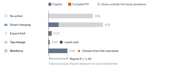
An estimated effect does not yet choose a mitigation measure, because the mitigation measures that remove the most hours also cost the most. A recommendation is therefore judged by its total cost. The total cost of mitigation measure \(a\) for query \(q\) is
\[ C_q(a) = c_{\mathrm{cap}}(a) + c_{\mathrm{e}} E_q(a) + \mu Y_q(a), \tag{6.27}\]
where \(c_{\mathrm{cap}}(a)\) is the annualised capital cost of the mitigation measure, \(E_q(a)\) the PV energy it curtails at a value \(c_{\mathrm{e}}\) per unit, and \(Y_q(a)\) the hours outside the band that remain at a penalty \(\mu\). The regret of a recommendation is the cost it forgoes relative to the best mitigation measure,
\[ \mathrm{Reg}_q = C_q(\hat a_q) - \min_{a \in \mathcal{A}} C_q(a). \tag{6.28}\]
Figure 6.12 shows the parts of the cost and the regret for one transformer of the case base.
Four policies were compared on the test transformers by their regret (Table 6.8). The case-based policy estimated the cost of every mitigation measure from the ten nearest kept cases and chose the least. The violation-pattern rule of Part 5 applied a tap change to over-voltage, smart charging to under-voltage, reinforcement to both and no action to neither. The remaining two applied a tap change everywhere and nothing anywhere. The violation-pattern rule had the least mean regret, 0.19, and chose a mitigation measure of least cost for 87% of the transformers. The case-based policy had a regret of 0.25 and chose optimally for 54%. Applying a tap change everywhere cost 1.93 in regret, more than taking no action, 1.55, because it deepens every evening under-voltage.
Figure 6.13 compares the policies. The rule derived from the violation patterns of Part 5 outperformed retrieval on this population because the least-cost measure is determined largely by the kind of violation, which the rule reads directly, whereas the case-based policy estimates four costs, each with an error, and its choice inherits the largest of them. A learned policy is therefore justified where the kind of violation leaves the choice undetermined, and any learned policy is compared with the rule it would replace before it is adopted, by the regret that Equation 6.28 defines.
The violation-pattern rule performed well because the mitigation measures of the case base act on the violation patterns by construction, the tap change on the midday rise and smart charging on the evening charging. Chapter 4 examines whether the rule holds on a network whose violations depend on more than these two terms, where the case-based policy has the advantage of requiring no such rule.
A policy that minimises the cost of each transformer separately says nothing about how its benefits and burdens are shared across the network, which the next section addresses.
Equity of Targeting
Recommendations made transformer by transformer can concentrate their effects. A programme that enrols the transformers of greatest benefit may serve a few networks only, and the volt-watt response of inverters curtails the customers at the ends of feeders more than those near the transformer. Measuring this concentration requires an index of inequality. For a burden \(\mathbf{b} = (b_1, \dots, b_m)\) shared among \(m\) units with mean \(\bar b\), the Gini coefficient is [40]
\[ G(\mathbf{b}) = \frac{1}{2 m^2 \bar b} \sum_{i=1}^{m} \sum_{j=1}^{m} |b_i - b_j|. \tag{6.29}\]
It is zero when the burden is shared equally and approaches one when a single unit bears it all. For ranked lists, fairness of exposure applies the same idea to the attention \(w_i\) of Equation 6.13 that each group receives [31].
An index only describes the concentration, and equity becomes an objective when the index is bounded. A programme of \(M\) places then chooses the set \(S\) of units of largest benefit subject to a bound \(\bar g\) on the Gini coefficient of the enrolment rates \(\boldsymbol{\phi}_S\) of the groups,
\[ \begin{aligned} S^\star = {} & \arg\max_{|S| = M} \textstyle\sum_{i \in S} \tau_i \\ & \text{subject to } G(\boldsymbol{\phi}_S) \le \bar g. \end{aligned} \tag{6.30}\]
Sweeping \(\bar g\) traces the price of equity, the benefit forgone for each reduction of \(G\).
The price was measured on a smart-charging programme that enrolled 20 of the 150 test transformers, with the hours removed as its benefit. The benefit rose with the length of the feeders, from a mean of 0.27 hours on the urban network to 1.17 hours on the most rural, so the unconstrained programme enrolled the rural networks, at a Gini coefficient of 0.258 across the four networks (Figure 6.14, Table 6.9). Bounding the coefficient at 0.1 reduced it to 0.095 and retained 96.3% of the hours removed. The price of near-equal enrolment was therefore 3.7% of the benefit.
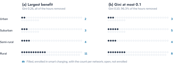
Figure 6.15 traces the frontier. Bounds of 0.3 and looser cost nothing, because the unconstrained programme already satisfies them, and the bound of 0.1 costs 3.7% of the hours removed. The frontier states the price of each degree of equity in the unit of the benefit, so that the choice of a bound becomes a decision of policy taken with its cost known rather than a property of the ranking.
Every result of this chapter, from the coverage of the radius to the price of equity, was computed against simulated outcomes. The final section makes explicit what this changes relative to the evaluation practised in recommender systems.
Evaluation Against a Simulator
The steps of the chain combine into a policy \(\pi\), which maps the features of a query to an action, and a policy is judged by its value, its mean cost over \(N\) queries. Recommender systems estimate this value offline from a log in which action \(a_i\) was taken with propensity \(\rho_{a_i}(\mathbf{x}_i)\), by inverse propensity weighting [21], [22],
\[ \hat V(\pi) = \frac{1}{N} \sum_{i=1}^{N} \frac{\mathbb{1}\{\pi(\mathbf{x}_i) = a_i\}}{\rho_{a_i}(\mathbf{x}_i)}\, C_i(a_i). \tag{6.31}\]
The estimate uses only the queries on which the policy agrees with the log, and its variance grows as the propensities fall. A simulator removes both limitations, because every action can be applied to every query,
\[ V(\pi) = \frac{1}{N} \sum_{i=1}^{N} C_i\bigl(\pi(\mathbf{x}_i)\bigr). \tag{6.32}\]
Figure 6.16 contrasts the two on six transformers of the case base.
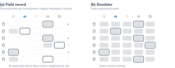
The mean regret of Table 6.8 is \(V(\pi)\) less the value of the policy that always chooses the cheapest mitigation measure, and the error of an uplift estimate in Table 6.7 is computed in the same way. Exact evaluation is not complete evaluation, however, and two limitations remain. A simulated outcome is only as accurate as the network model and the profiles that drive it, so a method is validated against the simulator rather than against the network. The methods are also trained on simulated cases, which a utility would replace with its records, and performance on records that mix field outcomes with confounded choices of action is the harder test, which Table 6.7 only begins.
Pitfall: the value of a policy estimated on the record that chose its actions
A recommender fitted on a utility’s record and evaluated on the same record is credited with the choices of the utility. Where the utility applied reinforcement to the worst transformers, a recommender that learns to recommend reinforcement for transformers like those appears to agree with good decisions, whatever the outcome of reinforcement was. The value of a policy must be estimated on cases whose actions were not chosen by the policy being evaluated, either by inverse propensity weighting, Equation 6.31, with the propensities of the utility, or by simulation, Equation 6.32, which needs no propensity.
Further Applications of Recommendation to Customers
The chain of this chapter was stated for transformers and mitigation measures, but its causal step applies wherever a utility chooses which customers receive an offer. The choice of households for a time-of-use tariff, a programme of demand response or managed charging is a recommendation in the sense of Equation 6.20: the action is the offer, the outcome the consumption at the hours the offer targets, and the uplift the change the offer causes in each household.
The Low Carbon London trial supplies a record in which both conditions of identification hold by design. Households were assigned at random to a flat tariff or to a dynamic time-of-use tariff for 2013, under which they were notified a day ahead of half-hours at a High price, so that the assignment depended on no feature of the household, Equation 6.23 holds, and every household had the same propensity, Equation 6.24. For the 1,079 households with readings in 2012 and 2013, 212 of them in the time-of-use arm, the outcome is the relative change of a household’s consumption in the High-price half-hours against the same half-hours of days without a High price, and the features describe its readings of 2012, before the trial: its mean demand, the share of its consumption in the evening and overnight, the ratio of its peak to its mean, and its variability.
The average effect was large and certain. Consumption in the High-price half-hours fell by 3.8% in the time-of-use arm and rose by 5.4% in the flat arm, whose households received no signal, an effect of 9.2 percentage points (Mann-Whitney \(p = 5.7 \times 10^{-26}\)). The effect is larger than the reduction of 3.5% that Part 7 estimates for the same trial, because it is a mean over households rather than the response of the median household, and its baseline is every day of the year without a High price rather than the ordinary days nearest to each event; the two estimates answer different questions, the total reduction a programme obtains and the response of a typical customer. Whether the effect differs between households is the question that targeting depends on. The T-learner and X-learner of Equation 6.25 and Equation 6.26 were fitted on one half of the households and ranked the other half by their estimated effect, and because the arms were randomised, the difference between the arms within the quarter ranked most responsive is an unbiased estimate of the effect in that quarter. Over twenty random halvings, the quarter ranked most responsive by the X-learner reduced its consumption by 12.1 points, with a 5th to 95th percentile of 9.3 to 15.9, against 8.0 points for the remaining three quarters, and the quarter exceeded the rest in 95% of the halvings; the T-learner reached 11.4 against 8.2 points, and exceeded the rest in 85% (Figure 6.17).
For a utility, the result means that the readings of a year before an offer identify households that respond about half as much again as the average, so that an offer limited to a quarter of the customers obtains more reduction per offer than an offer made to all. The gain is moderate, because five features of a year of readings describe habits rather than the reasons for which a household responds, and the variability between halvings shows that a single random split would overstate or understate it. The ranking also carries the risk that the equity bound of Equation 6.30 is meant to control: if the most responsive households are those with the most flexible demand, a programme limited to them offers the benefit of a lower bill to the households that already find it easiest to obtain. The same design applies to the selection of households for managed charging, where Part 7 detects the households that charge a vehicle and the uplift is the evening demand that managed charging moves, and to the selection of households for a battery, which Chapter 4 discusses.
Conclusion
This chapter stated retrieval, ranking and recommendation for the LV network as one decision chain. A query is described by its features, its outcome is estimated from the cases nearest to it, the queries are placed in an order, and each is assigned the mitigation measure of least estimated cost. Each step was given a formal statement, drawn from information retrieval, recommender systems and causal inference, and an evaluation that a simulator makes exact. Each was illustrated on a synthetic case base of 600 transformers whose outcome under five mitigation measures was known.
The case base answered the three questions of the introduction in turn. An estimate from similar cases can be trusted within a conformal trust radius, which admitted 89.9% of in-distribution queries over 200 splits at a nominal 90%, and 51.3% of queries from networks with longer feeders, whose refused queries were estimated with errors a third larger than the trusted ones. An adaptive error interval held the same coverage with intervals 24% narrower than a fixed width. An order is judged by measures that weight the top of the list, and by these the estimate of the nearest cases reached an NDCG at 10 of 0.858 over 200 splits, and a ranker learned for the purpose ranked significantly worse, with the largest difference over the whole list. A tap change that adds 0.29 hours on average appeared to add 1.26 hours when estimated naively from a record in which it followed the PV share, and the meta-learners removed most of this bias. Judged by cost, the violation-pattern rule of Part 5 chose the least-cost mitigation measure for 87% of transformers, in a case base where the mitigation measures act on the violation patterns by construction.
The limitations are those of a synthetic case base. Its outcomes follow a stated voltage model with four features and one unobserved strength of the voltage rise, and its networks differ only in the length of their feeders. The relative performance of the methods on it is therefore illustrative, not a result about real networks. Chapters 2 and 3 apply retrieval and ranking to the AusNet networks, where the outcomes come from power-flow simulation and the features from smart-meter data.
Exercises
- Change \(\alpha\) in the
setupcell from 0.1 to 0.2 and to 0.05. How do the trusted share and the interval width of Table 6.4 follow \(\alpha\), and does the coverage over repeated splits in Table 6.5 follow \(1 - \alpha\)? - Draw the queries of the shifted population with feeders between 1.2 and 2.4 times the original range. How do the trusted share and the error of the refused queries change?
- Make the choice of the tap change in the
upliftcell depend on \(\kappa\), the unobserved strength of the voltage rise, as well as on the PV share. Which condition of Equation 6.23 is then violated, and which estimators of Table 6.7 remain close to the simulated effect? - Raise the capital cost of reinforcement in
umeme.casebase.LEVERSfrom 1.5 to 3.0. How do the regret and the optimal share of the violation-pattern rule and of the case-based policy change?