| Population | Meters | Interval | Period | Region | Labels used |
|---|---|---|---|---|---|
| AusNet | 342 | 30 min | One year | Victoria, Australia | None; faults injected |
| Low Carbon London | 1,284 | 30 min | 2013 | London, United Kingdom | Price events; 228 households on the dynamic tariff |
| GoiEner | 1,000 | 60 min | June 2021 to May 2022 | Basque Country, Spain | None |
| GoiEner PV register | 662 | 60 min | June 2021 to May 2022 | Basque Country, Spain | PV self-consumption; 141 registered |
Meter Data Quality and Customer Behaviour
Chapter 1 formulated anomaly detection as a test of the hypothesis that an observation was drawn from the distribution of normal observations (Equation 10.2), and evaluated its methods on a synthetic population in which every anomaly was known. A distribution network operator holds no such population. It holds the readings of its meters, a register of the connections of its customers, and the records of the programmes in which those customers take part, and it must decide from them which readings to trust, which customers have connected generation that it does not know of, and whether a customer responded to a price. Each of these is a question of anomaly detection on measured data, and each departs from the synthetic case in what is known: the readings contain departures whose cause is uncertain, some labels exist but are incomplete, and the normal behaviour changes with the season.
This chapter applies the theory of Chapter 1 to three measured populations and to problems of this kind. The first is the validation of meter readings, where the rules of the industry are fixed-threshold tests whose false-alarm rate depends on the meter, and where the conformal threshold of Equation 10.26 meets its guarantee only while the days remain exchangeable. The second is the threshold of a detector shared by customers of different demand, for which the demand clusters of Part 5 provide the groups of the Mondrian threshold of Equation 10.30. The third is the detection of PV and of EV charging behind an import meter, problems in which the anomalies are common enough to violate the assumption of rarity on which density-based detectors rest. The fourth is the verification of the response of households to a price event, a contextual anomaly whose estimation requires the potential outcomes of Part 6.
Three findings recur. The false-alarm rate of a rule or a threshold depends on properties that a single setting does not capture: the resolution of the register, the interval of the readings, the level of demand and the season. Event features, which Chapter 1 found invariant to the timing of normal variation (Equation 10.20), were again the most informative representation, of a faulty day and of a meter with PV behind it. A baseline of ordinary days attributes to an event every change that it does not anticipate, including a bias of the estimator itself, and a control group is the means by which such changes are separated from the effect of interest.
Meter Data and Customer Behaviour in the Literature
The readings of smart meters pass through validation, estimation and editing before they are used for billing or analysis. Validation applies rules for implausible values, such as zeros, unchanged readings and readings beyond the rating of the connection; estimation replaces the readings that fail, and editing records the replacement. Chen and colleagues reviewed the dimensions of the quality of consumption data, among them completeness, accuracy and consistency, and the causes of their failure in metering and communication [1]. Peppanen and colleagues treated estimation as imputation and showed that methods exploiting the correlation between meters and between days outperform interpolation for gaps of more than a few readings [2]. The detectors of Chapter 1 complement the rules: a rule tests a property that a reading must have, whereas a detector tests whether a day resembles the normal days of its meter [3]. A register records energy in steps of fixed size, and the rounding of a continuous quantity to such steps is the subject of the theory of quantisation [4], which explains how often a register repeats a reading without a fault.
The guarantee of a conformal threshold rests on exchangeability, and its behaviour without it has been characterised recently. Barber and colleagues bounded the excess of the error rate of a conformal method over its target by a weighted sum of the distances between the distribution of each calibration observation and that of the test observation, and showed that weights favouring recent observations reduce the bound under gradual change [5]. Tibshirani and colleagues treated the case of a known change of the distribution of the inputs [6].
The register of connected generation is incomplete in many networks. Generation installed without notification is invisible to the operator, which then underestimates the export at midday and the demand that the generation masks. Shaker, Zareipour and Wood estimated the output of such sites from the measured output of a representative subset of known sites [7]. Zhang and Grijalva detected residential PV from the net load of individual meters and estimated its capacity [8], and Tabone, Kiliccote and Kara disaggregated the generation behind individual meters in real time [9]. Detection without labels in a population where PV is common meets the problem of masking, in which a group of similar outliers conceals each of its members from a method that compares a point with its neighbours [10], [11].
The verification of demand response rests on a baseline, the consumption that the customer would have had without the event. Coughlin and colleagues compared baselines built from the average of recent days and from regression on temperature [12]. For residential customers, Wijaya, Vasirani and Aberer showed that the bias of a baseline transfers money between the customer and the operator, and Mohajeryami and colleagues measured the errors of common baselines on residential data [13], [14]. The Low Carbon London trial tested a dynamic time-of-use tariff on households with a control arm on a flat tariff; Ozaki examined the willingness of its participants to shift their practices, and Yunusov and Torriti estimated the distributional effects of such tariffs on its data [15], [16]. The comparison of a treated group with a control group before and after a change is the difference-in-differences estimator of the causal effect, valid under the assumption that both groups would have changed alike without the treatment [17], [18].
Problem Formulation and Notation
The chapter uses the notation of Chapter 1 (Table 10.1) and extends it with the quantities of measured meters (Table 11.1). A meter records the energy \(e_{i,t}\) consumed by customer \(i\) in interval \(t\) of length \(\Delta t\), 30 minutes or one hour, as a reading rounded to the step \(\delta\) of its register, here 1 Wh:
\[ x_{i,t} = \delta \left\lfloor \frac{e_{i,t}}{\delta} + \frac{1}{2} \right\rfloor . \tag{11.1}\]
The readings of a day form the vector \(\mathbf{x}_{i,d}\) of Chapter 1, with \(T = 48\) or \(T = 24\) readings.
A validation rule is a statistic \(R(\mathbf{x})\) of a day and a fixed level \(m\) at which it flags the day, such as the length of the longest run of identical readings and a run of two hours. In the terms of Equation 10.2, the rule is a test of the hypothesis that the day is normal, and its false-alarm rate is the probability \(P_0\{R(\mathbf{x}) \ge m\}\) under the distribution of normal days. Unlike the conformal threshold of Equation 10.26, the level \(m\) is not calibrated on the meter, so the false-alarm rate of a rule is a property of the meter and its load that the rule does not control. A self-baseline detector of Chapter 1, by contrast, sets its threshold from the calibration days of the meter itself.
Three further settings recur. In the first, the unit of detection is a meter rather than a day: a meter with PV behind it is an anomaly of the population, scored against the other meters, and the share \(\pi\) of such meters enters the precision of Equation 10.6. In the second, the threshold is set per group \(z\) of meters, the demand clusters of Part 5, as in Equation 10.30. In the third, the anomaly is the effect of a known event. With \(Y_{i,d}(1)\) and \(Y_{i,d}(0)\) the consumption of household \(i\) in the window of the event on day \(d\) with and without the price signal, as the potential outcomes of Part 6, the effect of the event on the household is
\[ \tau_{i,d} = \frac{Y_{i,d}(1)}{Y_{i,d}(0)} - 1 , \tag{11.2}\]
of which only one outcome is observed, so that \(Y_{i,d}(0)\) must be estimated from a baseline.
| Symbol | Description |
|---|---|
| \(e_{i,t}\), \(x_{i,t}\), \(\delta\) | Energy of customer \(i\) in interval \(t\), its reading, and the step of the register |
| \(\Delta_t\), \(f_\Delta\), \(\sigma\) | Change of the energy between consecutive intervals, its density, and its spread |
| \(p_i\), \(\rho_i\) | Probability that meter \(i\) repeats a reading, and its ratio of repeats to changes of one step |
| \(R(\mathbf{x})\), \(m\) | Statistic of a validation rule and the level at which it flags a day |
| \(c_t\), \(g_t\), \(r_i\) | Consumption and PV generation behind an import meter, and the ratio of midday to evening import |
| \(Y_{i,d}(1)\), \(Y_{i,d}(0)\), \(\tau_{i,d}\) | Consumption with and without the price event, and the effect of the event |
| \(b_{i,d}\), \(\Delta_{i,d}\), \(\hat\rho_d\) | Baseline of ordinary days, the observed relative change, and the estimated response |
Data and Protocol
Table 11.2 lists the populations. The AusNet population holds the half-hourly demand of 342 households over one year, the readings on which Parts 5 and 6 are built. The Low Carbon London population holds the half-hourly consumption of 1,284 households in 2013, 228 of which were on the dynamic time-of-use tariff of the trial and the remainder on a flat tariff.1 The GoiEner population holds the hourly consumption of 1,000 meters of a Basque energy cooperative from June 2021 to May 2022, drawn as in Part 5, and a second sample of 662 meters of the same cooperative, of which 141 are registered with PV self-consumption and the remainder are residential meters without it.2 The registered meters record only the energy imported from the network.
The data hold three kinds of label. The price signal of the London trial gives the half-hours of every price event and the arm of every household. The register of GoiEner gives the meters with PV behind them, as declared to the cooperative; a meter without a declaration may nevertheless have PV, so the label is complete for the positives and uncertain for the negatives. No dataset records the faults of its meters. The evaluation of detectors of faults therefore follows Chapter 1: faults of stated kind are injected into measured days, and the detector is evaluated on held-out normal days and on the injected days with the AUC of Equation 10.5. The natural departures in the readings are reported as they are, with their possible causes, but not used to evaluate a detector, since their cause is not known.
The protocol of each experiment states which days fit a detector, which calibrate its threshold and which test it. Where the days are drawn at random from the year, the calibration and test days are exchangeable, the condition of Equation 10.27. Operation does not draw days at random: a detector fitted on past days is applied to the days that follow, and the calibration of thresholds over time is examined explicitly. Where two methods are compared on the same households or splits, the comparison is reported with a Wilcoxon signed-rank test over them [19].
Validation of Meter Readings
Validation is the first use of anomaly detection on meter data, and the one an operator applies to every reading. This section examines the rules of validation on the natural departures of the three populations, derives the rate at which a register repeats a reading without a fault, proposes a statistic that separates chance repeats from a frozen register, and then evaluates the self-baseline detectors of Chapter 1 on measured days, including the calibration of their thresholds over time.
Rules for Implausible Readings
A validation rule flags a day with a stated property: zero readings over several hours, a reading that does not change over several intervals, or a reading far above the usual level of the meter. Each property has more than one cause (Figure 11.1). An unchanged reading is the signature of a frozen register, a fault, but a register that advances in steps of 1 Wh also records the same value in consecutive intervals when the load is small and steady. A day of zero readings may be an outage, an absence of the occupants with every appliance switched off, or a reading lost in communication and replaced by zero.
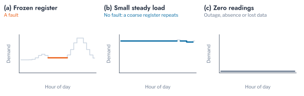
Table 11.3 reports the departures that five rules flag in the three populations. Their frequency differs widely between the populations. Zero readings for three hours or more occurred on at least one day for 19.9% of the AusNet meters, 7.7% of the London meters and 28.4% of the GoiEner meters, and on 0.3%, 1.1% and 6.4% of all days. Identical readings for two hours or more occurred for 33.6%, 38.0% and 81.6% of the meters. Read as tests of Equation 10.2, the rules have false-alarm rates that differ by an order of magnitude between populations, since no fault is known to explain more than a fraction of these flags. A rule set once for every meter of a network therefore sends inspectors to very different shares of the meters of different populations, and its threshold must be set for the population, or for the type of meter, on which it is applied.
The rule for high readings shows the same difficulty from the other direction. A reading above 20 times the median of its meter occurred for 33.0%, 43.5% and 51.0% of the meters, on 2.4%, 6.0% and 5.9% of all days. Such readings are the signature of a register error, but also of an electric heater, an oven or a charging vehicle in a household whose median load is small, and the rule cannot separate the two without the history of the household. Rules remain the first step of validation because they are transparent, simple to compute and auditable, properties that a settlement process requires. Their limitation is that each fixes its level in advance, independently of the meter, and the remainder of this section derives what that level implies for meters of different resolution and load.
Chance Repeats of a Register
The rate at which a register repeats a reading without a fault follows from Equation 11.1. Two consecutive readings are equal when the change \(\Delta_t = e_{i,t} - e_{i,t-1}\) of the underlying energy rounds to zero. For a density \(f_\Delta\) of the change that is smooth on the scale of \(\delta\),
\[ P(x_t = x_{t-1}) = \int_{-\delta/2}^{\delta/2} f_\Delta(u)\,\mathrm{d}u \approx \delta\, f_\Delta(0) , \tag{11.3}\]
and if the change is normal with standard deviation \(\sqrt{2}\,\sigma\), as for two independent readings of spread \(\sigma\),
\[ P(x_t = x_{t-1}) \approx \frac{\delta}{2\sqrt{\pi}\,\sigma} . \tag{11.4}\]
The probability of a repeat is therefore proportional to the step of the register and inversely proportional to the spread of the change, which grows with the energy recorded in an interval. Table 11.4 confirms the dependence: readings of up to 20 Wh repeated the previous reading in 8.4%, 12.0% and 28.7% of cases in the three populations, and readings above 100 Wh in 0.9%, 1.3% and 1.6%. The hourly GoiEner meters record smaller readings relative to their step, 18.9% of their readings lying at or below 50 Wh against 11.3% for AusNet, and repeat more often at every level.
Figure 11.2 compares the observed probability of a repeat with two predictions. The Gaussian model of Equation 11.4, with the spread estimated from the changes in each band, has the slope of the observations but lies below them by a factor of two to five, because the change of a steady load is concentrated near zero more sharply than a normal density. The general form of Equation 11.3 requires no model of the density: a change of one step in either direction has probability \(\delta f_\Delta(\pm\delta)\), which for a smooth density is close to \(\delta f_\Delta(0)\), and the observed repeats lie close to that level throughout. The repeats of the three populations are thus almost all consistent with chance, at a rate set by the energy per interval.
A rule flags a run of \(m\) consecutive repeats. If each reading of a meter repeated the previous one independently with probability \(p_i\), the probability of at least one such run in a day of \(T\) readings would be approximately
\[ P\{R(\mathbf{x}) \ge m\} \approx 1 - \bigl(1 - (1 - p_i)\, p_i^{\,m}\bigr)^{T - m} , \tag{11.5}\]
which falls geometrically with \(m\). Figure 11.3 shows that the observed share of flagged days falls far more slowly. For runs of two hours, independence predicts 0.05% of AusNet days and 0.26% of London days, against 1.0% and 1.9% observed, and the gap widens with the length of the run. A steady load repeats in runs, because the change between intervals is itself correlated, so a rule calibrated on independent repeats flags many days without a fault. Restricting the rule to readings above 50 Wh, 50 steps of the register, reduced the share of GoiEner days flagged from 12.0% to 4.2% (Table 11.3), but 67.7% of its meters still had such a run at least once.
Pitfall: a validation rule transferred between meters
A rule of validation embodies an assumption about the meter: its interval, the step of its register and the level of the load it records. The same rule applied to meters of another interval or another population flags a different share of days for reasons unrelated to faults, as Equation 11.3 and Equation 11.5 make explicit. The level of a rule is set per class of meter, and the share of days flagged is monitored as a property of the rule as well as of the meters.
A Statistic of Repeated Readings
The argument of Equation 11.3 yields a statistic that adapts to the meter. For each meter, the ratio of repeats to changes of one step,
\[ \rho_i = \frac{\#\{t : x_{i,t} = x_{i,t-1}\}}{\tfrac{1}{2}\,\#\{t : |x_{i,t} - x_{i,t-1}| = \delta\}} \approx \frac{f_\Delta(0)}{f_\Delta(\delta)} , \tag{11.6}\]
is close to one when repeats arise by chance from a smooth density of changes, whatever the level of the load and the step of the register. A frozen register adds a share \(\pi_{\mathrm{s}}\) of repeats that the density of changes does not explain, so that \(\rho_i \approx 1 + \pi_{\mathrm{s}} / (\delta f_\Delta(\delta))\) exceeds one. The statistic compares a meter with the chance level implied by its own readings, as the self-baseline detector of Chapter 1 compares a day with the days of its own meter.
Table 11.5 evaluates the statistic on 100 clean and 100 faulty meters per population, into which 5 or 15 stuck days were injected, against the rule of a two-hour run. The median ratio of the clean meters was 1.11, 1.12 and 1.19, close to the value of one that chance predicts. With 15 stuck days, the ratio attained an AUC of 0.972, 0.899 and 0.848 and the rule 0.956, 0.918 and 0.713. With 5 stuck days, the rule was superior on the half-hourly meters of AusNet and London (0.879 and 0.854 against 0.814 and 0.763), whose stuck runs are long relative to their chance runs, and the ratio on the hourly GoiEner meters (0.618 against 0.583). Figure 11.4 shows the distributions. The ratio is thus not more sensitive than the rule on the meters for which the rule was designed; its advantage is that it transfers to meters of another interval and level without a new setting.
Self-Baseline Detection of Injected Faults
A self-baseline detector, fitted on the days of one meter, flags days that depart from the normal days of that meter. It complements the rules of validation, since a fault that preserves every property a rule tests, such as a drift of the level or an under-recording of every reading, is a departure from the history of the meter rather than an implausible value. The detectors of Chapter 1 were applied to 60 households of each of the AusNet and London populations. For each household, 200 days fit the detector, 60 calibrate its threshold, 40 normal days are held out, and five kinds of fault are injected into ten further days: a spike, a register stuck at one reading, a dropout to zero, a drift of the level and an under-recording of half of every reading.
Table 11.6 reports the AUC of the local outlier factor of Equation 10.11 for the five representations of a day of Chapter 1. Events with statistics attained the highest mean AUC on both populations, 0.772 on AusNet and 0.791 on London, against 0.611 and 0.623 for the readings themselves, the ranking that Chapter 1 found on days whose normal variation includes randomly timed activations. The events detected a stuck register (AUC 0.922) and a dropout (0.969), whose runs of unchanged or zero readings they count directly through the event vector of Equation 10.22, whereas the readings themselves attained 0.548 and 0.673, because a run of ordinary values at an unusual time resembles the variation of normal days. No representation detected the under-recording reliably: an under-recorded day has the shape and timing of a normal day at a lower level, within the range of normal days of a household whose consumption varies between days by a factor of two or more. Its detection requires a measurement that the meter does not control, the energy entering the transformer, which Chapter 3 treats through the energy balance.
Figure 11.5 compares the ten detectors of Chapter 1 on the events with statistics of the AusNet households. The one-class support vector machine of Equation 10.14 attained the highest mean AUC, 0.786, followed by the local outlier factor (0.771), the kernel density estimate (0.763) and the control limit of Equation 10.7 (0.758); COPOD attained the lowest, 0.699. The differences were consistent across households: the one-class support vector machine exceeded the local outlier factor by 0.015 (Wilcoxon \(p = 0.008\) over 60 households) and the control limit by 0.028 (\(p < 10^{-9}\)). They were nevertheless smaller than the differences between representations, 0.087 between the best and the worst detector against 0.161 between the events with statistics and the readings for the same detector. On measured days, as on the synthetic population, the representation of a day decides more of the result than the family of the detector. An operator who builds a detector of faulty meters therefore gains more from the choice of the features of a day, events and their statistics rather than the raw readings, than from the choice among detectors, which can be made for simplicity of computation.
The threshold converts a score into a decision at the target false-alarm rate \(\alpha\) of Equation 10.27. Figure 11.6 shows the share of normal and faulty days flagged by the conformal threshold of the local outlier factor at targets from 2% to 20%. The false-alarm rate on the held-out normal days was 1.0%, 3.8%, 7.4% and 17.8% at targets of 2%, 5%, 10% and 20%, below the target in each case, as Equation 10.27 guarantees for exchangeable days and as the tied scores of count features make conservative (Equation 10.29). The dropout was flagged on 87% to 100% of its days and the stuck register on 53% to 90%, while spikes, drift and under-recording were flagged on 4.5% to 47% of their days, little more often than normal days at the same target. A lower target therefore costs little detection of the faults that the representation separates, and cannot recover the faults it does not.
Calibration over Time
The guarantee of Equation 10.27 holds when the calibration days and the test days are exchangeable. The days of a year are not: demand changes with the season, and a detector calibrated on the first months of a year is applied to the months that follow. Barber and colleagues bounded the excess of the false-alarm rate over its target in this case. For a threshold calibrated on \(n\) days, the false-alarm rate of a new day satisfies
\[ \Pr\{ s(\mathbf{x}) > \tau \} \le \alpha + \sum_{j=1}^{n} \tilde{w}_j\, d_{\mathrm{TV}}\bigl(\mathbf{s},\, \mathbf{s}^{(j)}\bigr) , \tag{11.7}\]
where \(\mathbf{s}\) is the vector of the scores of the calibration days and the new day, \(\mathbf{s}^{(j)}\) the same vector with calibration day \(j\) and the new day exchanged, \(d_{\mathrm{TV}}\) the total-variation distance between their distributions, and \(\tilde{w}_j = 1/(n+1)\) for the unweighted threshold [5]. Under exchangeability every distance is zero and Equation 10.27 is recovered; under a change of season the distances grow with the time between the calibration days and the new day.
The threshold of each of the 60 households of each population was calibrated at a target of 10% in two ways. In the first, 200 training, 60 calibration and 100 test days were drawn at random from the year. In the second, the training days were the first 200 days, the calibration days the following 60 and the test days the last 100, as in operation. Figure 11.7 shows the false-alarm rate of each household. With days drawn at random, the mean rate met the target for both representations and both populations, between 9.4% and 10.1%. With test days that followed the calibration days, the mean rate of the London households rose to 17.5% with the readings and 12.5% with the events, and the standard deviation across households reached 12.4 and 10.6 percentage points. On AusNet the mean rate remained near the target, 9.9% with the readings and 8.3% with the events, but the rate of individual households ranged widely about it, with a standard deviation of 7.8 and 5.8 points. Event features were less affected than the readings, since a count of events is less sensitive to a change of level. A false-alarm rate verified on days drawn at random from the year therefore overstates the reliability of a threshold in operation, where it is applied to days that follow its calibration, and a utility must verify the rate on days that follow the calibration, as the bound of Equation 11.7 requires.
Equation 11.7 suggests the remedy: calibration days close in time to the test days reduce the distances. Figure 11.8 compares three rules on the last 100 days of the year, in blocks of 20 days. With the threshold fixed after the first calibration, the false-alarm rate of the London households rose from 14% to 22% as the winter approached, with a mean of 17.5% and a standard deviation across households of 12.4 points. Recalibrating the threshold on the 60 days before each block held the mean at 13.5% and reduced the standard deviation to 6.0 points; refitting the detector as well gave 15.0% and 5.7 points. On AusNet, recalibration left the mean unchanged, 10.0% against 9.9%, and reduced the standard deviation from 7.8 to 4.7 points. Recalibration on recent days, the unweighted form of the recency weights that Barber and colleagues proposed, does not restore the guarantee, but it narrowed the spread of false-alarm rates across households by 40% to 50% at the cost of no additional model. Recalibration on a rolling window of recent days is therefore the practical default for an operator, since it costs only the storage of recent scores.
Thresholds per Demand Cluster
An operator with many meters may fit one detector on the days of all of them rather than one detector per meter, which requires fewer models and uses the variation between households as a reference. Its threshold then serves households of very different demand, and Chapter 1 showed on the synthetic population that a single threshold distributes the false alarms unevenly between groups. The Mondrian threshold of Equation 10.30 calibrates one threshold per group \(z\) on the calibration scores of that group alone,
\[ \tau_z = s^{(z)}_{\left(\lceil (n_z + 1)(1 - \alpha) \rceil\right)} , \tag{11.8}\]
the order statistic of the \(n_z\) calibration scores of group \(z\), and bounds the false-alarm rate within each group, provided that the days are exchangeable within it. The groups must be known before the score is computed and must hold enough calibration days for the order statistic to be stable; the demand clusters and the archetypes of Part 5 satisfy both conditions.
One Isolation Forest was fitted on the statistics of the days of all 342 households, with 200 training, 60 calibration and 105 test days drawn at random from the year, and the procedure was repeated over 20 splits. Table 11.7 reports the false-alarm rate and the detection of a 50% under-recording by demand cluster. At a target of 10%, the single threshold produced a false-alarm rate of 20.2% in the cluster of high demand, 4.3% in the cluster of medium demand and 3.6% in the cluster of low demand; the threshold per cluster produced 9.8%, 9.6% and 9.7%. At a target of 5%, the rates of the single threshold were 11.8%, 1.4% and 0.6%, and those of the thresholds per cluster 4.9%, 4.7% and 4.9%. The largest departure of a cluster from the target, averaged over the splits, was 10.3 percentage points with the single threshold and 1.1 with the thresholds per cluster (Wilcoxon \(p < 10^{-5}\) over the 20 splits). A single threshold therefore concentrates the false alarms, and the inspections they cause, on the customers of high demand, at twice the target rate, while it misses faults in the other clusters; a threshold for each cluster, Equation 11.8, distributes the inspections as the target intends.
Figure 11.9 adds the thresholds per archetype of Part 5, which group households by the shape of their demand rather than its level. They reduced the largest departure only to 7.8 percentage points, with false-alarm rates of 17.7%, 5.0% and 5.6% in the clusters of high, medium and low demand. The score of the pooled detector depends mainly on the level of a household’s consumption, and a Mondrian threshold equalises the false-alarm rate only across groups that stratify the score; the choice of groups is therefore a modelling decision, informed by what the score measures.
The redistribution of false alarms changed what the detector could find. A detector fitted on the population scores a day by its departure from the days of all households, and the days of households of high demand lie in the tail of that distribution, so the single threshold spends most of its false alarms on them and leaves the households of low demand with a threshold that their days rarely approach. With the threshold per cluster, the detection of a 50% under-recording in the cluster of low demand rose from 11.6% to 25.1% at a target of 10%, and in the cluster of medium demand from 4.5% to 11.8%, while in the cluster of high demand it fell from 4.3% to 1.3%. The total number of false alarms is approximately the same under both rules, 9.8% and 9.7% of the days of the population; the threshold per cluster allocates them so that each cluster receives its share. The demand clusters of Part 5 serve here as a stratification of the population for the purpose of calibration, a use that does not depend on whether the clusters are stable as segments of behaviour.
Behind-the-Meter PV
PV installed without notification to the operator is a departure from the register of the network rather than a fault of a meter. It changes the export at midday, the voltage at the connection and the demand that the network appears to supply, and an operator that does not know of it underestimates both the hosting capacity consumed and the demand that the generation masks. This section uses the register of GoiEner as labels and examines whether the readings of an import meter identify the meters with PV behind them, without using the labels to fit the detector.
The Signature of PV in Import Readings
An import meter at a household with PV records the consumption \(c_t\) less the generation \(g_t\) only where the difference is positive,
\[ x_t = \max(c_t - g_t,\, 0) , \tag{11.9}\]
and the export, where generation exceeds consumption, goes unrecorded (Figure 11.10). The signature of PV is therefore a fall of the import around midday, to zero on clear days when the array exceeds the load, and not a negative reading. Its strength follows from Equation 11.9. With a midday consumption \(c_{\mathrm{m}}\) and an evening consumption \(c_{\mathrm{e}}\), the ratio of midday to evening import of meter \(i\),
\[ r_i = \frac{\bar{x}_{i}(\text{11:00 to 16:00})}{\bar{x}_{i}(\text{19:00 to 23:00})} = \frac{\mathbb{E}\bigl[\max(c_{\mathrm{m}} - g,\, 0)\bigr]}{c_{\mathrm{e}}} \le \frac{c_{\mathrm{m}}}{c_{\mathrm{e}}} , \tag{11.10}\]
falls from the ratio of the household’s own consumption towards zero as the generation grows relative to the midday load, and rises again in winter, when the generation is lower.
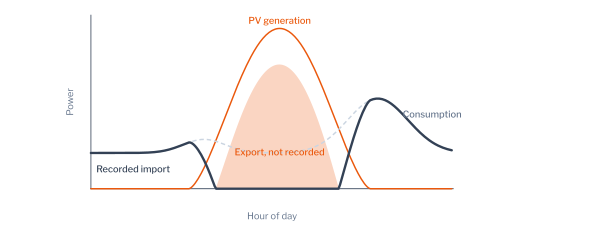
Figure 11.11 shows the median daily import of the 141 registered meters and the 521 meters without PV, each divided by its own daily mean. The registered meters imported less in the midday window than in the morning and evening, in summer and in winter; over the year, the median registered meter imported 0.58 of its daily mean from 11:00 to 16:00 and 0.99 overnight, whereas the median meter without PV imported 1.11 and 0.68. The median of the mean daily ratio of Equation 11.10 over June was 0.49 for the registered meters and 1.12 for the others, and over December 0.65 and 1.08, as the model predicts for lower winter generation.
The signature has causes other than PV. A household that is absent during the day and active in the evening has a low ratio, and a household with storage heating charged overnight has a high one. Figure 11.12 shows the summer ratio of every meter: most registered meters lie below the meters without PV, but the two groups overlap. The detection of PV from import readings is therefore the detection of meters whose pattern resembles that of PV meters, among which some have another explanation, and its results are candidates for inspection rather than conclusions.
Unsupervised Detection and Masking
Each meter was represented by its year of hourly import in five ways: the mean day, the shape of the mean day divided by its peak, statistics of the year including the ratio of Equation 11.10, event features of the daylight hours in which the meter imports at its own lowest level, and the events with the statistics. The event features count the episodes in which the import falls to the floor of the meter during daylight, their duration and their hour, the events that Equation 11.9 predicts for PV. Two detectors, Isolation Forest (Equation 10.15) and the local outlier factor (Equation 10.11), scored each meter against all others, without labels. The evaluation used the 141 registered meters among 662, a share of 21%, and 20 draws in which the registered meters were sub-sampled to 5%, a share closer to that of unregistered PV in a network.
Table 11.8 reports the AUC and the precision among the \(k\) meters of highest score, \(k\) being the number of registered meters. At a share of 5%, Isolation Forest on the events with statistics attained an AUC of 0.948 and a precision of 0.491: of the meters it ranked highest, about half were registered PV, against 5% at random. The mean day attained 0.922 and 0.446, the statistics 0.930 and 0.417, and the shape of the mean day 0.821 and 0.130; the shape discards the level of import, and with it the information that the midday import of a PV meter is low in absolute terms. The precision at the share of 21% was higher for every method, 0.709 for the best, although the AUC changed little. Equation 10.6 of Chapter 1 explains the difference: at a fixed recall and false-alarm rate, the precision rises with the prevalence \(\pi\), so that the same detector appears more useful in a population where the anomaly is common.
The local outlier factor behaved otherwise: at the share of 21% its AUC was 0.527 to 0.732, against 0.719 to 0.916 for Isolation Forest. The cause is masking (Figure 11.13). By Equation 10.11, the score of a point is the mean ratio of the local reachability densities of its \(k\) nearest neighbours to its own. When the registered meters number more than \(k\) and resemble one another, the \(k\) nearest neighbours of a registered meter are other registered meters of the same density, every ratio is close to one, and its score falls to that of a normal meter. Isolation Forest is less affected: by Equation 10.15, a group of \(n_{\mathrm{a}}\) similar points that lies apart from the remaining \(n_{\mathrm{s}} - n_{\mathrm{a}}\) is separated from them after a number of random splits of the order of \(\log_2(n_{\mathrm{s}}/n_{\mathrm{a}})\), so its points keep shorter paths than the normal points as long as the group remains a minority.
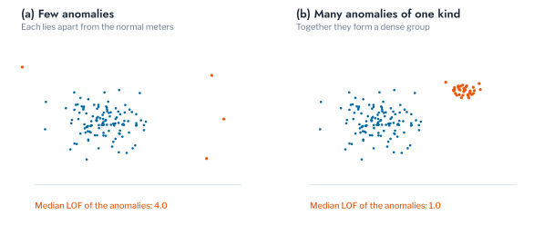
Figure 11.14 tests this account by varying the number of registered meters among the 521 meters without PV. With up to 10 registered meters, every detector attained an AUC between 0.923 and 0.947. As the registered meters outnumbered the 20 neighbours of the local outlier factor, its AUC fell to 0.875 with 27 registered meters, 0.815 with 57 and 0.709 with 141. With 100 neighbours it fell later and less, to 0.859, and Isolation Forest remained between 0.908 and 0.935 throughout. The number of anomalies relative to the neighbourhood of a density-based detector is thus a property of the problem that determines the suitable detector, and a population in which a kind of anomaly is common, as PV is in some networks, is better treated as a population of two groups than as a population with outliers.
Of the 141 meters that Isolation Forest on the events with statistics ranked highest in the full sample, 41 were not registered with PV. Their ratio of midday to evening import in summer was above the median of the registered meters, 0.32, for all but four of them; the median ratio of the meters without PV was 0.98. These four meters are candidates for inspection as unregistered PV. The remaining 37 depart from the population for other reasons, and their inspection would establish whether the departure is of interest to the operator.
Behind-the-Meter EV Charging
A vehicle charged at home without notification is the counterpart of unregistered PV in the evening. Part 5 found that EV adoption raises the loading of a transformer in proportion to its customers and lowers the voltage at the end of its feeders, and Part 6 ranked transformers for reinforcement by the charging they would carry, so an operator that cannot see the chargers already connected underestimates the evening risk it ranks. The import meter records charging directly, unlike PV export, but as part of the household’s demand, and the question is whether the readings alone separate the households that charge.
No dataset of the book records which households charge a vehicle at home: GoiEner registers nine meters on the Spanish super-valley tariff for vehicles, none of them over the study year. The recorded charging of 200 vehicles (data.evsessions), each a year of half-hourly power at up to 14.8 kW, was therefore added to the measured readings of a share of the AusNet households, one vehicle per owner. The label is semi-synthetic, but both the demand and the charging are measured, so the detector faces the variation of real households and real vehicles. The representations are those of the PV problem, with charging events in place of daylight events: runs of readings at least 3 kW above the household’s median demand, summarised by the event vector of Equation 10.22 (Figure 11.15).
Table 11.9 reports the detection. At a share of 5%, Isolation Forest on the charging events attained an AUC of 0.984 and a precision of 0.665 among the highest-ranked meters, and the statistics of the year 0.963 and 0.335. The mean day reached only 0.764 and 0.071, and the shape of the mean day 0.432, below chance. The ordering follows the invariance argument of Chapter 1 (Equation 10.20). A vehicle is charged at different hours on different days, so averaging the year spreads its blocks across the evening and leaves a mean day that resembles a household with a large evening load, whereas the count, duration and depth of the charging events do not depend on when the blocks fall. Normalising by the peak removes the level of charging as well, and the shape is then uninformative. For the detection of vehicles behind the meter, an operator should therefore represent each meter by its charging events rather than by its mean day, which is the representation most often used for segmentation.
Masking appeared again. At a share of 20%, the local outlier factor fell below chance on the charging events (0.424), the statistics (0.465) and the shape (0.354), while Isolation Forest kept 0.928 on the charging events, the behaviour that Equation 10.11 predicts once the owners outnumber the neighbourhood of 20 and form a dense group of their own. For an operator, the implications are those of the PV problem with one difference. Behind-the-meter PV and EV charging are both detectable from readings already collected, by a detector chosen for a population in which the technology is common rather than rare, and the highest-ranked meters are candidates for inspection, at a precision that Equation 10.6 ties to the share of owners. The difference is the season: charging is present all year and in the evening, so a meter that acquires a vehicle shows the change at once, which Chapter 3 treats as a change of behaviour rather than an anomaly.
Verification of Demand Response
A price event asks customers to reduce or increase their consumption over a stated window, and the operator or the supplier must establish how much they did. The question is one of a contextual anomaly with a known context: the consumption in the window of an event is compared with the consumption expected for that window without the event. The London trial provides 74 days with High-price events and 102 days with Low-price events in 2013, with 752 and 1,624 event half-hours, and the arms of its households.
Baselines and the Control Arm
The unobserved outcome \(Y_{i,d}(0)\) of Equation 11.2 is estimated by a baseline, here the mean over the \(k = 10\) ordinary days nearest to \(d\) of the same day type, weekday or weekend, with \(E_{i,d'}(W)\) the energy of household \(i\) in window \(W\) on day \(d'\):
\[ b_{i,d} = \frac{1}{k} \sum_{d' \in \mathcal{N}_k(d)} E_{i,d'}(W_d) . \tag{11.11}\]
The observed relative change of the household on the event day is
\[ \Delta_{i,d} = \frac{E_{i,d}(W_d)}{b_{i,d}} - 1 , \tag{11.12}\]
which equals the effect \(\tau_{i,d}\) of Equation 11.2 plus the error of the baseline as an estimate of \(Y_{i,d}(0)\). The median of \(\Delta_{i,d}\) over the households of an arm thus contains a bias whenever the median error of the baseline is not zero. The control arm, whose tariff did not change, has \(\tau_{i,d} = 0\), so its median change measures that bias directly. The response to the price on day \(d\) is estimated as the difference between the median changes of the two arms,
\[ \hat{\rho}_d = \operatorname{median}_{i \in \mathrm{ToU}} \Delta_{i,d} - \operatorname{median}_{i \in \mathrm{Std}} \Delta_{i,d} , \tag{11.13}\]
a difference-in-differences that removes the bias common to both arms (Figure 11.16). It identifies the response under the assumption that, without the price, the median errors of the baselines of both arms would have been equal,
\[ \operatorname{median}_{i \in \mathrm{ToU}} \Bigl( \tfrac{Y_{i,d}(0)}{b_{i,d}} - 1 \Bigr) = \operatorname{median}_{i \in \mathrm{Std}} \Bigl( \tfrac{Y_{i,d}(0)}{b_{i,d}} - 1 \Bigr) , \tag{11.14}\]
the assumption of parallel trends [17], which the random assignment of households to the arms of the trial makes plausible and which can be checked on days without an event.
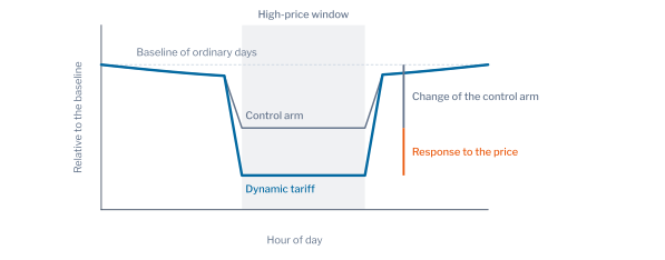
Table 11.10 reports the results. In the High-price half-hours, the median household on the dynamic tariff consumed 8.6% less than its baseline, and the median household of the control arm 4.6% less. The response to the price was a reduction of 3.5%, with a bootstrap interval over event days of 3.0% to 4.6%. A baseline alone would have attributed to the price a reduction more than twice as large as the response. In the Low-price half-hours, both arms consumed less than their baselines, 2.0% and 3.8%, and the response to the price was an increase of 2.6% (1.8% to 3.6%), which the baseline alone would have reported as a reduction. A programme of demand response that pays customers on the evidence of a baseline alone would therefore pay for a reduction about twice as large as the one the price caused, and the payment rule must include a control group, as Equation 11.14 assumes.
Table 11.11 examines the source of the bias. On ordinary days drawn at random, with the windows of the High events, the median change was −4.9% on the dynamic tariff and −5.3% in the control arm, and on the ordinary day before each event −3.6% in both. The bias is therefore not a property of the event days but of the estimator: a household’s consumption in a window of a few hours is right-skewed across days, so the ratio of one day to the mean of ten has a median below one. The ratio of the summed energies of an arm to the sum of its baselines does not carry this bias: in the control arm it departed from its baseline by only 0.2% on the event days, and on the dynamic tariff by 5.8%. The difference of the arms was 0.8 and 0.2 percentage points on the two kinds of day without an event, consistent with Equation 11.14. The median and the ratio of sums answer different questions, the change of the typical household and the change of the total consumption, and the latter, a reduction of 4.7% against the control arm, is the quantity on which the value of the programme to the network depends.
Figure 11.17 shows how the estimates depend on the number \(k\) of ordinary days in the baseline. The change of each arm moved with \(k\): with one day, the ratio of two single days is nearly symmetric and the control arm changed by −0.2%; with 20 days it changed by −5.5%. The response, the gap between the arms, remained between −2.4% and −4.2% for the High price and between 2.2% and 2.9% for the Low price. Figure 11.18 shows the two arms on every event day: the control arm moved from day to day, and the dynamic tariff lay to the left of it on nearly every High-price day and to the right on most Low-price days. The control arm is the means by which the day-to-day movement and the bias of the estimator are both removed. An operator that evaluates a programme should therefore keep a randomly chosen group of customers outside it, since no choice of baseline days removes the bias that the control group removes.
Responses of Individual Households
The aggregate response does not establish which households responded. For each household, the mean of \(\Delta_{i,d}\) over the 74 High events was compared with its distribution under the null hypothesis of no response, obtained by applying the same windows to ordinary days drawn at random, \(B = 1{,}000\) times. The p-value of household \(i\), with \(\bar{\Delta}_i\) the observed mean and \(\bar{\Delta}_i^{(b)}\) the mean of draw \(b\), is
\[ p_i = \frac{1 + \#\{b : \bar{\Delta}_i^{(b)} \le \bar{\Delta}_i\}}{1 + B} , \tag{11.15}\]
the conformal p-value of Equation 10.28 with the placebo draws in the role of the calibration days. Under the null hypothesis it is uniform, and the Benjamini-Hochberg procedure of Equation 10.31 selects the households at a false-discovery rate of 10%. The test was repeated after subtracting from every change the median change of the control arm on the same day, as in Equation 11.13.
Table 11.12 reports the shares selected. Without the control arm, 14.9% of the households on the dynamic tariff were selected as responding, and 0.7% of the households of the control arm; with the control arm subtracted, 16.2% and 0.9%. The household test was little affected by the bias of the estimator, because its null distribution, drawn from ordinary days, carries the same bias, and because the variation of a single household between ordinary days in the window of the first High event, a coefficient of variation of 0.44 to 0.84 across the interquartile range of households, far exceeds the common change of 4.6%. Figure 11.19 shows the distribution of the p-values: uniform in the control arm, as the null hypothesis requires, and with an excess of small values on the dynamic tariff, from which the procedure selects about one household in six.
The two levels of verification answer different questions. The aggregate response, with its control arm, answers how much the programme reduced demand, the quantity on which the value of the programme to the network depends. The household test answers which customers can be relied upon, the quantity that targeting and the design of a future programme require. The selected households are anomalies in the sense of Chapter 1, departures from the normal days of a household at known times, and the control of the false-discovery rate is what makes a list of them usable; the households not selected may have responded inconsistently or by an amount that their variation conceals, so the share selected is a lower bound on the share that responded.
Further Applications of Meter Analytics
The problems of this chapter share one structure: a quantity that the meter does not record directly, a faulty register, a PV array, a vehicle or the response to a price, is inferred from the signature it leaves in the readings, and the inference is tested against a label where one exists. The same structure serves three further problems of a distribution network operator.
The first is the detection of heat pumps behind an import meter. A heat pump adds a demand that rises as the outdoor temperature falls and that runs for long periods in the morning and the evening of cold days. Its signature is therefore the dependence of the daily energy on the temperature rather than a block of high demand, and the representation by events used for electric vehicles is replaced by the slope of daily energy against heating degree days. The masking found for behind-the-meter PV, where a detector fitted on a population with many adopters learns the adopters as normal, applies in the same way as adoption grows, and a reference population without heat pumps, or a threshold per demand cluster as in Equation 11.8, is required.
The second is the detection of supply interruptions from the readings. A meter that records zero consumption over consecutive intervals on several meters of one feeder indicates an interruption of supply rather than a fault of the meters, and the chance-repeat model of Equation 11.6, which separates genuine repeated readings from a frozen register, separates a run of zeros at one meter from simultaneous runs on a feeder. The coincidence across meters is the evidence, as the coincidence of export is in the network chapters in preparation.
The third is the identification of the phase to which a customer is connected, which a distribution network operator often does not record reliably. The voltage of meters on the same phase moves together, and the correlation of each meter’s voltage with the voltage of the phases at the transformer assigns it to a phase; a meter whose correlation departs from the others of its assigned phase is flagged with the conformal threshold of Chapter 1. Chapter 6 of Part 5 treats this problem as constrained clustering, and this chapter supplies its validation.
Conclusion
This chapter applied the theory of Chapter 1 to the measured readings of three populations and to four problems of a distribution network operator. Validation rules, read as tests of Equation 10.2 with an uncalibrated level, flagged shares of meters that differed by a factor of more than two between populations, from 33.6% to 81.6% for identical readings over two hours. The rounding of the register explained the difference: the probability of a chance repeat is proportional to the step of the register and inversely proportional to the spread of the change of the load (Equation 11.3), and runs of repeats are far more frequent than independence predicts. The ratio of repeats to changes of one step (Equation 11.6) was close to one on clean meters in all three populations, and it detected stuck registers on the hourly meters where the run rule failed. Self-baseline detection on measured days ranked the events with statistics first, with mean AUC 0.772 and 0.791 on AusNet and London; the choice among ten detectors changed the mean AUC by less than the choice of representation, and no method detected under-recording reliably.
The conformal threshold met its target when calibration and test days were exchangeable and exceeded it when the test days followed them, by 7.5 percentage points on average for the readings of London households, as the bound of Equation 11.7 allows. Recalibration on the most recent days reduced the spread of false-alarm rates across households by 40% to 50%. A single threshold for a detector fitted on all AusNet households produced a false-alarm rate of 20.2% in the cluster of high demand and 3.6% in the cluster of low demand at a target of 10%, and Mondrian thresholds per demand cluster of Part 5 brought each cluster to between 9.6% and 9.8% and doubled the detection of under-recording among households of low demand, whereas thresholds per archetype did not equalise the clusters.
On the register of GoiEner, unsupervised detection identified meters with PV behind them from import readings alone, with an AUC of 0.948 and a precision of 0.491 at a share of 5% for Isolation Forest on daylight events with statistics. The local outlier factor lost its accuracy once the PV meters outnumbered its neighbourhood, the masking that Equation 10.11 predicts. On the London trial, the response to a High price was a reduction of 3.5% for the median household against a change of 8.6% that a baseline alone would have reported; the difference was a bias of the median of ratios, present on ordinary days as well, which the control arm removes and the ratio of summed energies avoids. About one household in six on the dynamic tariff was selected as a consistent responder at a false-discovery rate of 10%.
The limitations follow from the labels. The faults of the meters were injected, with stated magnitudes, because no dataset records them. The register of PV is complete only for its positives, and the meters ranked highly without a registration could not be verified. The baselines of the London trial used ordinary days without a model of the weather. Chapter 3 addresses the faults that a meter cannot reveal about itself, through the energy balance between the meters and their transformer, together with inverter faults and the changes of behaviour after which the models of Parts 5 and 6 require refitting.
Exercises
- Derive Equation 11.4 from Equation 11.3 for two independent readings of spread \(\sigma\), and compute the probability of a repeat for a steady load of 40 Wh per interval with \(\sigma = 2\) Wh. Compare it with the band of Table 11.4 that contains this level.
- Lower the energy floor
FLOORin thesetupcell to 0.02 kWh and recompute Table 11.3. Which population’s share of flagged days changes most, and how does Equation 11.5 explain the change? - Show from Equation 11.6 that a meter that repeats one reading for \(h\) hours a day, every day, has a ratio that grows linearly in \(h\). Verify the slope in the
repeatratiocell by injecting stuck runs of two and of six hours. - In the
recalibrationcell, calibrate on the 30 days before each block rather than 60. How do the mean and the spread of the false-alarm rate of the London households change, and which term of Equation 11.7 does the change act on? - Replace the demand clusters in the
mondriancell by terciles of each household’s mean demand. Do the terciles, which stratify the level of demand directly, equalise the false-alarm rate of Table 11.7 as well as the demand clusters? - In the
maskingcurvecell, set the number of neighbours of the local outlier factor to 50. At what number of registered meters does its AUC begin to fall, and how does the answer relate to the argument from Equation 10.11? - Compute the response of Table 11.10 with the ratio of summed energies for the Low price, and explain from the skewness of household consumption why the median of ratios and the ratio of sums differ.
UK Power Networks, SmartMeter Energy Consumption Data in London Households, London Datastore, with the price schedule of the trial in
Tariffs.xlsx, https://data.london.gov.uk/dataset/smartmeter-energy-use-data-in-london-households.↩︎GoiEner, GoiEner smart meters data, Zenodo, https://doi.org/10.5281/zenodo.7362094; the register of self-consumption is the field
self_consumption_typeof its metadata, types 41, 42 and 43 under Royal Decree 244/2019.↩︎