Retrieval for Connection Requests
Chapter 1 stated retrieval for the Low Voltage (LV) network and tested it on a synthetic case base whose outcomes followed a voltage model of four features. On that case base the nearest cases estimated a new transformer’s hours outside the band with a mean absolute error of 1.17 hours, and a conformal trust radius refused most of the queries drawn from networks with longer feeders. Both results rested on the model that generated the cases, in which the features that drive the outcome are known and measured. On a real network neither holds by construction. The features available to a Distribution System Operator (DSO) are those of its smart meters, its asset register and its network model, the outcome follows from a power flow, and the population of a new request may differ from the one the case base was built on in ways the features do not record.
This chapter applies retrieval to the AusNet networks of Part 5, in the form of a decision a DSO takes routinely: whether to approve a request to connect rooftop Photovoltaic (PV) without a network study, which retrieval answers from simulated customers that resemble the request. The chapter asks which features make a retrieved estimate accurate enough to approve or refuse a connection, when the trust radius detects that an estimate should not be used, and how a decision can be given a guaranteed rate of error. Chapter 3 takes up the second decision of the planning stage, the order in which transformers enter a programme of work.
Retrieval in Distribution Planning
Estimating the effect of a new connection without a full study is the purpose of the hosting capacity methods of distribution planning. Stochastic methods simulate many placements of PV on a feeder and report the share of placements that violate a limit [1], and surveys of the field distinguish these from deterministic, optimisation-based and streamlined methods by their cost and their reliance on a network model [2]. Model-free and clustering-based estimates have been proposed for networks whose models are incomplete [3], [4]. These methods estimate the capacity of a feeder or a transformer, whereas a request concerns one connection point, and the voltage at a point depends on the impedance between it and the transformer. The voltage rise caused by a connection that injects active power \(P_q\) and reactive power \(Q_q\) through a Thevenin impedance \(R_q + jX_q\) at nominal voltage \(V\) is approximately
\[ \Delta V_q \approx \frac{R_q P_q + X_q Q_q}{V}. \tag{7.1}\]
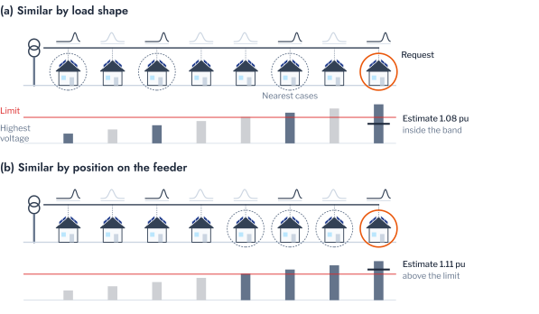
The approximation makes the position of a connection a candidate feature for retrieval, alongside the shape and size of demand that Part 5 used to group customers. Figure 7.1 contrasts the two. Customers of similar shape may stand anywhere on a feeder, whereas the customers nearest in position share the impedance of Equation 7.1.
The evaluation of a retrieval on real data raises two further questions, the design of the split and the shift of the population. Customers of a network are not independent cases. Several customers are assigned the measured load profile of the same household, and all customers of a transformer share its rating and its upstream impedance. A random split of customers therefore places near-duplicates of a test case in the case base, a form of leakage that inflates the measured accuracy [5]. Roberts and colleagues showed that data with hierarchical or spatial structure require blocked splits that hold out whole groups [6], and the groups here are the transformer and the household. A model may also be applied to queries whose distribution differs from that of its training data, either in the features or in the relation of the outcome to the features [7]. Conformal guarantees assume exchangeability and fail under such a shift, unless the calibration is reweighted for a known change in the features [8] or made separately within each group, as in Equation 6.10. Whether the trust radius of Equation 6.5 detects a given shift is therefore an empirical question, which the sections that follow answer after stating the quantities that retrieval estimates.
Clusters in the Decision Chain
Part 5 grouped the households of AusNet by the shape and by the level of their demand, and the violations of HPK11 by their duration, depth and timing. A natural expectation is that these groups predict the outcomes this part estimates and orders, and the evidence of this chapter is that they do not (Table 7.1). The voltage of a connection is set by its position on the network: the transformer and the impedance at the connection point explained 90.8% of the variance of every customer’s highest voltage, and the midday demand of its household, with a median of 0.42 kW against a 5 kWp array, added nothing. Customers are moreover assigned the profiles of households independently of their position, so that the archetype explained 0.03% of the variance of the impedance. On HPK11 the history of over-voltage is no better a predictor: among the 35 transformers that exceeded 1.10 pu at 20% PV, their hours at 20% and at 80% agreed with a Kendall’s \(\tau_b\) of 0.010.
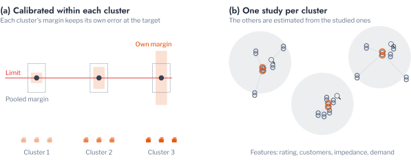
Clusters nonetheless serve the decisions, as structure rather than as predictors, which is also how recommender systems use them: to scale to large catalogues, to serve new users and to treat groups of users equally [9]. This part uses them in three roles (Figure 7.2), two of which this chapter takes up. As strata, the demand clusters define the groups within which a guarantee of the error of a decision is calibrated, so that it holds for every segment of customers rather than on average, as Equation 6.10 requires [10]. As representatives, clusters of transformers identify the few transformers whose study best covers the others, the competence that case-based reasoning seeks in a case base [11]. As groups of a programme, the constraints that the violation patterns separate, thermal and voltage, define separate rankings, because their mitigation measures differ, as asset management ranks by failure mode [12]. The third role is the subject of Chapter 3, and Chapter 4 adds two further roles, a mitigation measure recommended for each violation pattern and the equity of curtailment across the demand clusters.
Labelled Risk Sets
A labelled risk set assigns to each customer of a network its outcomes under a stated adoption, and the features that are known before any study. Four sets were simulated with popo on the AusNet network models of Part 5 (Table 7.2). Each customer was given a 5 kWp array with inverters set to the AS/NZS 4777.2 Australia A volt-VAr and volt-watt characteristics. With \(v_q(t)\) the voltage at its connection point in half-hour \(t\) of a clear summer day, its voltage outcome is the highest voltage of the day,
\[ y_q^{\mathrm{v}} = \max_t v_q(t). \tag{7.2}\]
Each customer was separately given a 7.36 kW charger in use from 18:00 to 21:00. With \(p_q(t)\) its demand, including the charger, on the day of highest evening demand, the network peaks in the half-hour
\[ t^\star = \arg\max_t \sum_j p_j(t), \tag{7.3}\]
and the thermal outcome of the customer is its contribution to that peak,
\[ y_q^{\mathrm{t}} = p_q(t^\star). \tag{7.4}\]
The voltage outcome decides a connection directly, by comparison with the upper limit \(\overline{v} = 1.10\) pu of AS 61000.3.100. The thermal outcome is a contribution, which a DSO compares with the remaining headroom of the transformer.
The first set covers HPK11, each of whose 5,274 residential customers is assigned the measured load profile of one of the 342 AusNet households, and the second CRE21, the second urban network of the same models, with 3,374 customers on 70 transformers. The third and fourth keep HPK11 and its assignment of customers to transformers but replace the AusNet households with households of London and of the Basque Country (GoiEner), each on a summer day of its own record and excluding households whose demand exceeds 20 kW. The four sets thus differ in two controlled ways. CRE21 changes the network and keeps the households, and the London and GoiEner sets change the households and keep the network. On HPK11 34.9% of customers exceeded \(\overline{v}\), against 20.2% on CRE21, although the median impedance at the connection point was almost equal, 0.076 and 0.077 \(\Omega\).
The features of a customer form four groups,
\[ \mathbf{x}_q = \bigl(\mathbf{s}_q, \mathbf{m}_q, \mathbf{a}_q, R_q, X_q\bigr). \tag{7.5}\]
The shape \(\mathbf{s}_q\) holds the first three principal components of its household’s mean day, each day normalised by its own peak, fitted on the AusNet households. The size \(\mathbf{m}_q\) holds the mean demand, the mean daily evening peak between 17:00 and 21:00 and the mean demand between 10:00 and 15:00. The asset features \(\mathbf{a}_q\) are the rating of its transformer and the number of single-phase customers it supplies. The position is the resistance \(R_q\) and reactance \(X_q\) of the Thevenin impedance at the connection point, obtained from a fault study of the network model. The shape and the size are known from the smart meter and the asset features from the register. The position requires a model of the LV network, which not every DSO holds, but it requires no power flow under the new connection.
Table 7.3 collects the quantities of the chapter, extending the notation of Chapter 1 (Table 6.2).
| Symbol | Description |
|---|---|
| \(q\), \(\mathbf{x}_q = (\mathbf{s}_q, \mathbf{m}_q, \mathbf{a}_q, R_q, X_q)\) | A query, a requested connection, and its features: shape, size, assets and position |
| \(v_q(t)\), \(y_q^{\mathrm{v}}\), \(\overline{v}\) | Voltage at the connection point, its daily maximum, and the upper limit of 1.10 pu |
| \(p_q(t)\), \(t^\star\), \(y_q^{\mathrm{t}}\) | Demand of the customer, half-hour of the network peak, and the contribution to it |
| \(\mathcal{T}\), \(\mathcal{T}^{+}\), MAE, MA | Test customers, those above the limit, mean absolute error, rate of missed refusals |
| \(\hat\sigma_q\), \(\lambda\), \(\hat\lambda\), \(L_i(\lambda)\), \(\hat R(\lambda)\) | Spread of the nearest outcomes, margin and its calibrated value, loss and empirical risk of a margin |
| \(\alpha\), \(n^{+}\), \(z\) | Target error, calibration customers above the limit, and a group of customers |
Retrieval of the Risk of a New Connection
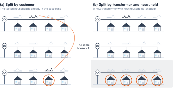
A request to connect is a query from a customer whose household may not have been simulated, on a transformer that may not have been studied, and the evaluation reproduces this position (Figure 7.3). Each split held out 20% of the transformers and, independently, 20% of the households, and tested only customers on a held-out transformer whose load profile comes from a held-out household. A second 20% of each calibrated the trust radius and the intervals, and customers on the remaining transformers with the profiles of the remaining households formed the case base \(\mathcal{D}_1\). The split was repeated 200 times.
Pitfall: a split by customer
A random split of the customers places customers of the same transformer, and customers who replay the same household, in both the case base and the test set. The nearest case of a test customer is then a neighbour on its own feeder or the same household on another one, and the error measures the recall of cases already simulated rather than the estimate for a new connection. The held-out unit must be the unit on which the method will be applied: here a transformer not yet studied and a household not yet simulated, held out together. The same rule applies to the calibration of the trust radius and of the margins, whose guarantees hold only for queries exchangeable with the calibration cases.
The estimate is the mean outcome of the 10 nearest cases of Equation 6.3, on features standardised over the case base. Four sets of features were compared, adding the groups of Equation 7.5 in turn, against four baselines. The population mean estimates every query by the mean of the case base. The archetype, demand-cluster and demand-tercile means estimate it by the mean of the customers of the same group of Part 5, the segmentations a utility would apply to a new customer. A linear regression on all features shows what a global model achieves with the same information, and a blend of the two, \(\beta \hat y_q^{\mathrm{kNN}} + (1 - \beta) \hat y_q^{\mathrm{lin}}\) with \(\beta\) chosen on the calibration customers, interpolates a retrieval with a parametric model as nearest-neighbour language models do [13]. Describing a new customer by its features rather than by its history is the remedy that recommender systems apply to the cold start, where factorisation machines add such side information to the identities of users and items [14]. Each method was scored by its mean absolute error over the \(n_{\mathrm{test}}\) test customers \(\mathcal{T}\) of a split,
\[ \mathrm{MAE} = \frac{1}{n_{\mathrm{test}}} \sum_{q \in \mathcal{T}} \lvert y_q - \hat y_q \rvert. \tag{7.6}\]
For the voltage, the error matters through the decision it implies. A connection is approved when its estimated highest voltage is within the limit, \(\hat y_q^{\mathrm{v}} \le \overline{v}\), and the costly error is the approval of a connection that exceeds it. Its rate among the over-limit customers \(\mathcal{T}^{+} = \{q \in \mathcal{T} : y_q^{\mathrm{v}} > \overline{v}\}\) is
\[ \mathrm{MA} = \frac{1}{\lvert \mathcal{T}^{+} \rvert} \sum_{q \in \mathcal{T}^{+}} \mathbb{1}\bigl\{\hat y_q^{\mathrm{v}} \le \overline{v}\bigr\}, \tag{7.7}\]
and the rate of refusals among the customers within the limit is defined in the same way.
The segmentations of Part 5 did not reduce the voltage error at all (Figure 7.4). The population mean erred by 7.88 mpu, or 1.8 V at 230 V, and the archetype, demand-cluster and tercile means by 7.89 mpu each. Nearest cases on the shape of demand were worse than the population mean, at 8.21 mpu, and adding the size of demand and the asset features brought them back only to 7.93 mpu. Adding the position halved the error, to 4.22 mpu or about 1.0 V, and the linear regression on the same features reduced it further, to 3.94 mpu, and the blend of the two to 3.86 mpu. For the thermal outcome the order was different. The demand-cluster mean, at 1.38 kW, improved on the population mean of 1.46 kW, nearest cases on shape alone were the worst estimate, at 1.74 kW, and each group of features reduced the error, to 1.26 kW with all four, against 1.22 kW for the linear regression and 1.20 kW for the blend.
The decisions followed the errors. Because the mean highest voltage, 1.095 pu, lies just within the limit, the population mean and every segmentation mean approved all of the over-limit connections, and nearest cases on shape and size approved 96.6% of them. With the position, the nearest cases approved 28.7% of the over-limit connections and refused 11.0% of those within the limit, and the linear regression 31.0% and 8.5%. An estimate from the position therefore removes most of the approvals that would breach the limit, at the cost of refusing about one connection in ten that would not, and a DSO could send the refused requests to a study rather than decline them.
These differences held split by split (Table 7.4). Adding the position reduced the voltage error by 3.72 mpu in all 200 splits, whereas adding the size of demand to its shape changed it by 0.005 mpu and reduced it in only 49.0% of the splits, with a Wilcoxon p-value of 0.978 [15]. For the thermal outcome the size of demand reduced the error by 0.158 kW in 86.5% of the splits. The linear regression improved on the nearest cases by 0.277 mpu and 0.034 kW, in 73.0% and 75.0% of the splits. The blend improved on the linear regression by 0.084 mpu in 65.5% of the splits, and by 0.021 kW on average although in only 46.0% of them, a gain concentrated in the splits in which the regression erred most. The voltage of a connection is therefore retrieved by where it stands rather than by how its household uses energy, as the variance decomposition of Part 5 anticipated, and its demand contributes to the thermal outcome through its size more than through its shape. That a linear regression improved on the nearest cases, and their blend on both, also indicates that the outcome varies smoothly with the position, as Equation 7.1 suggests, while the nearest cases correct it where it does not.
Choosing the Transformers to Study
The case base of a utility is built from the studies it can afford, and with thousands of transformers the choice of which to study determines how well the others are retrieved. The clustering of Part 5 offers one choice. The transformers are described by their rating, customers, impedance and demand, standardised, and clustered by k-means into as many clusters \(\mathcal{C}_1, \dots, \mathcal{C}_m\) as there are studies, with centres \(\boldsymbol{\mu}_k\); the transformer studied in each cluster is its medoid,
\[ j_k = \arg\min_{j \in \mathcal{C}_k} \lVert \mathbf{a}_j - \boldsymbol{\mu}_k \rVert, \tag{7.8}\]
where \(\mathbf{a}_j\) are the features of transformer \(j\). This is the competence that case-based reasoning seeks in a case base, a few cases that cover the others [11]. The medoids were compared with transformers drawn at random, for budgets from 4 to 20 of the 43 transformers, by the error of retrieval for the customers of the transformers not studied, over 40 repeats in which the households were also split in half, so that no household was both studied and retrieved.
The medoids improved on a random choice only modestly, and not at every budget (Figure 7.5). With 12 to 20 transformers studied they reduced the voltage error by 1.2% to 3.6%, to 4.26 mpu against 4.37 mpu at 20, and the thermal error by up to 2.8%. With 8 they were worse, at 5.70 mpu against 4.99 mpu. A medoid is a typical transformer, whereas retrieval for the others also needs the unusual ones, at the edges of the feature space, and with few studies the clusters cannot hold both. A selection that covers the extremes, by the distance of every transformer to the nearest one studied, is the alternative that the notion of competence suggests. A utility with a budget of a few studies should therefore spend them on the transformers least like those already studied, since the typical ones are the cases that retrieval estimates well without them.
These errors were measured on customers of the network the case base was built on. A request may come from a household unlike any simulated, or from another network, and the next section examines whether the trust radius recognises such requests.
Refusal Under Shift
The trust radius of Equation 6.5 refuses the queries that do not resemble the case base. Its calibration at \(\alpha = 0.1\) guarantees that at most 10% of exchangeable queries are refused, and the adaptive interval of Equation 6.9 that at least 90% of the trusted outcomes are covered. Both were calibrated on HPK11 with all features of Equation 7.5 and applied to the held-out HPK11 customers, to every customer of CRE21, and to the London and GoiEner customers on the held-out HPK11 transformers. A shift the radius detects lowers the share of queries trusted, and a shift it misses lowers the coverage of those it trusts. Figure 7.6 illustrates the two cases.
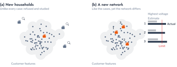
On the held-out HPK11 customers the radius trusted 87.7% of queries and the voltage interval covered 89.0% of the trusted outcomes (Figure 7.7). The trusted share fell slightly below the nominal 90%, as expected of queries that are new in two respects at once, and the coverage held. The households of other populations were refused more often, 20.8% of the London and 29.0% of the GoiEner queries, and the coverage of those trusted held at 88.3% and 87.7%. The radius therefore detected the change of households, conservatively, since the refused queries were estimated with errors only about 12% larger than the trusted ones. Single splits varied widely around these means, by more than ten points of coverage, which is why a conformal guarantee is read over repeated splits, as the remark of Chapter 1 states.
The change of network was not detected. The radius trusted 85.9% of the CRE21 customers, almost as many as of HPK11, but the voltage interval covered only 77.7% of their outcomes, and the error of the trusted queries rose from 4.25 to 5.48 mpu. The customers of CRE21 resemble those of HPK11 in every feature, including the impedance at the connection point, but the network responds differently, as the lower share of customers above \(\overline{v}\) shows. The relation between features and outcome had changed while the features had not, and a radius on the features cannot detect such a shift. The thermal outcome, which depends on the household more than on the network, was covered at 90.2% on CRE21. A model applied to a network on which it was not calibrated therefore requires the guarantee of Equation 6.10, with calibration cases from that network, and a few studies on each new network provide them. On the network of the case base, however, the radius guarantees only how often a resembling request is refused, not how often a trusted estimate leads to a wrong decision, which the next section addresses.
Decisions with a Guaranteed Error
The decision that matters to a DSO is whether to approve a connection, and with the position the nearest cases still approved 28.7% of the connections that exceeded the limit. This section calibrates the decision itself, so that its rate of error is bounded, and sends the requests on which the estimate is too uncertain to a network study.
The calibration follows conformal risk control [16], which extends the guarantee of split conformal prediction (Equation 6.6) from coverage to the expected value of any loss that does not increase as a decision becomes more cautious. Language models use the same construction to withhold generated claims until the rate of false ones falls below a target [17]. The uncertainty of an estimate is measured by the spread of the highest voltages of the \(k\) nearest cases of request \(q\),
\[ \hat\sigma_q = \Bigl( \frac{1}{k} \sum_{j \in \mathcal{N}_k(q)} \bigl( y_j - \hat y_q \bigr)^2 \Bigr)^{1/2}, \tag{7.9}\]
and a margin \(\lambda \ge 0\) is counted in units of this spread. A request is approved when its estimate, raised by the margin, is within the limit,
\[ \hat y_q + \lambda \hat\sigma_q \le \overline{v}, \tag{7.10}\]
and is otherwise sent to a study. The loss of a calibration customer \(i\) that exceeds the limit is whether it would have been approved,
\[ L_i(\lambda) = \mathbb{1}\bigl\{ \hat y_i + \lambda \hat\sigma_i \le \overline{v} \bigr\}, \tag{7.11}\]
which does not increase with \(\lambda\). Over the \(n^{+}\) calibration customers above the limit, its mean is
\[ \hat R(\lambda) = \frac{1}{n^{+}} \sum_{i=1}^{n^{+}} L_i(\lambda), \tag{7.12}\]
and the margin is the smallest whose corrected mean is at most the target \(\alpha\),
\[ \hat\lambda = \inf \Bigl\{ \lambda : \frac{n^{+}}{n^{+} + 1} \hat R(\lambda) + \frac{1}{n^{+} + 1} \le \alpha \Bigr\}. \tag{7.13}\]
If a new over-limit customer is exchangeable with those of the calibration set, the probability that it is approved is bounded by the target,
\[ \mathbb{E}\bigl[ L_{n^{+} + 1}(\hat\lambda) \bigr] \le \alpha. \tag{7.14}\]
A second rule also refuses. A request is decided automatically when the band of \(\lambda\) spreads around its estimate lies wholly on one side of the limit,
\[ \bigl| \hat y_q - \overline{v} \bigr| > \lambda \hat\sigma_q, \tag{7.15}\]
approved below it and refused above it, and is sent to a study otherwise. Its loss is a wrong automatic decision,
\[ L_i(\lambda) = \mathbb{1}\bigl\{ | \hat y_i - \overline{v} | > \lambda \hat\sigma_i \bigr\}\, \mathbb{1}\bigl\{ (\hat y_i > \overline{v}) \ne (y_i > \overline{v}) \bigr\}, \tag{7.16}\]
which also does not increase with \(\lambda\), and it is calibrated by Equation 7.13 over every calibration customer. Figure 7.8 illustrates both steps. This arrangement, in which an inexpensive estimate decides where it is certain and an exact computation is reserved for the remaining cases, corresponds to speculative decoding in language models, in which a small model proposes and a large one verifies [18].
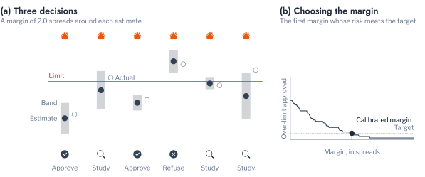
Both rules were calibrated on the calibration customers of each of the 200 splits, at targets from 1% to 20%, and applied to the test customers (Figure 7.9). The achieved error stayed at its target within sampling error. At \(\alpha = 0.10\) the first rule approved 9.8% of the over-limit connections and the second decided 9.4% of the requests wrongly, and at \(\alpha = 0.05\) the errors were 5.2% and 4.8%, with standard errors of the mean between 0.3 and 0.6 points. The guarantee is obtained at the cost of the requests sent to a study. To approve at most 5% of the over-limit connections, the first rule studied 57.1% of the requests, and at 10% it studied 47.8%; because it never refuses, every likely refusal is studied as well. The second rule studied 37.0% of the requests at an error of 5% and 19.0% at 10%. Since every request would otherwise be studied, a calibrated retrieval removed between 63% and 81% of the studies at a stated rate of wrong decisions. The guarantee rests on exchangeability, which Figure 7.7 showed to fail on another network, where the calibration must use customers of that network.
The guarantee of Equation 7.14 holds on average over the over-limit customers, and a segment of customers may bear more than its share of the error. With the demand clusters of Part 5 as strata, the margin can be calibrated within each cluster \(z\) on its own \(n_z^{+}\) over-limit customers,
\[ \hat\lambda_z = \inf \Bigl\{ \lambda : \frac{n_z^{+}}{n_z^{+} + 1} \hat R_z(\lambda) + \frac{1}{n_z^{+} + 1} \le \alpha \Bigr\}, \tag{7.17}\]
where \(\hat R_z\) is the mean loss of Equation 7.12 over the cluster, so that the guarantee holds within each cluster, as in Equation 6.10. At a target of 5%, the pooled margin approved 5.8% of the over-limit connections of the cluster of lowest demand and 5.6% of the cluster of highest demand, above the target, and 4.2% of the remaining cluster (Figure 7.10). Calibrated within each cluster, the margins approved 4.2%, 3.2% and 4.4%, within the target for every cluster, at the cost of studying between 68.0% and 73.9% of the requests rather than between 56.3% and 57.9%. A utility that must treat its customers equally can therefore buy a guarantee for each segment with roughly a quarter more studies.
Retrieval and its decisions serve a request for one connection. A reinforcement programme instead concerns every transformer of a network at once, which is a question of ranking.
Further Applications of Retrieval to Customers
Retrieval answered a connection request by the outcomes of the most similar simulated cases. The same principle answers a question that a retailer or a distribution network operator receives from customers: which tariff will cost this household less over the coming year. The outcome of a tariff for a household is its annual bill, which its readings determine exactly once the year has passed, and the problem is to predict the cheaper tariff from the readings available when the customer asks.
The flat-tariff households of the Low Carbon London trial supply a test of this problem with real prices. Their consumption in 2013 did not respond to the price signal, which they did not receive, so their bill under the trial’s time-of-use schedule follows from their readings, and their bill under a flat rate follows from their consumption. The flat rate is set to raise the same revenue from these 1,184 households as the time-of-use schedule, 13.83 pence per kWh, so that neither tariff is cheaper on average. Time-of-use was nevertheless cheaper for 40.1% of the households, and the annual saving ranged from a loss of £25.5 to a saving of £32.7 between the 5th and the 95th percentile, with a median loss of £2.1. A new customer is represented by its first four weeks of readings, its normalised daily profile and its mean level, and the tariff is recommended from the mean saving of its nearest households by Equation 6.3, each household held out in turn.
Retrieval recovered most of the saving that a fixed rule forgoes (Figure 7.11). Recommending the same tariff to every household forgoes £6.04 a year on average, for either tariff, because a revenue-neutral rate makes the gains of some households equal the losses of the others. The nearest household alone chose the cheaper tariff for 71.9% of the households, with a mean regret, Equation 6.28, of £1.61; twenty neighbours chose it for 78.2%, with a regret of £1.12, and forty did no better. Four weeks of readings therefore support a recommendation that is wrong for about one household in five, and wrong mostly for households whose two bills differ little, since the regret of a wrong choice is the difference between the bills.
For a utility, two qualifications follow from the theory of Chapter 1. The bills assume that a household does not change its consumption under the new tariff, whereas the households of the time-of-use arm reduced their consumption at High prices, so the recommendation understates the saving for the households that would respond, which the uplift of Chapter 1 estimates. The four weeks were in January, and a household whose consumption differs between seasons is represented by its winter alone; the trust radius of Equation 6.5 identifies the new customers whose readings lie far from every household of the case base, for which a recommendation should wait for more readings. The same retrieval serves the recommendation of an export limit or a battery to a household with PV, with the annual bill under each option computed from the readings of similar households.
Conclusion
This chapter applied retrieval to labelled risk sets of the AusNet networks, in which every customer was assigned its simulated voltage and thermal outcome together with the features known before a study. Retrieval was evaluated on transformers and households held out together, over 200 splits. The voltage of a new connection was retrieved by its position on the network. Nearest cases with the Thevenin impedance of the connection point erred by 4.22 mpu against 7.88 mpu for the population mean, and approved 28.7% of the connections that exceeded the limit, whereas the segmentations of Part 5 approved all of them. The thermal contribution was retrieved by the size of demand, with an error of 1.26 kW against 1.46 kW.
The trust radius detected a change of households and missed a change of network. It refused 20.8% and 29.0% of the queries from two other populations, but trusted 85.9% of the customers of CRE21, whose voltage intervals then covered 77.7% rather than 90% of the outcomes. A model transferred to a new network therefore requires calibration on that network. On the network of the case base, conformal risk control bounded the rate of wrong decisions: at a target of 5%, a rule that approves, refuses or studies made 4.8% wrong decisions while studying 37.0% of the requests. The clusters of Part 5 entered the chain as structure rather than as predictors. Calibrated within each demand cluster, the decision rule kept the approval error of every cluster within a target of 5%, where the pooled rule exceeded it in two clusters, at the cost of about a quarter more studies, and studying the medoids of clusters of transformers reduced the error of retrieval for the others by at most 3.6% against a random choice. Applied to customers rather than connections, the same retrieval recommended the cheaper tariff from four weeks of readings for 78.2% of the households of the Low Carbon London trial.
The limitations follow from the simulations. Customers are assigned the profiles of households independently of their position, so that the analysis cannot represent a network in which types of household cluster geographically. The risk sets fix one array size, one charger and one day for each outcome, and the replacement populations are placed on the AusNet network and irradiance, so the shift they represent is one of households rather than of climate. The position features require a model of the LV network, and where a DSO has none, a proxy such as the distance along the feeder would have to replace them. Chapter 3 turns from the estimate for one connection to the order of the transformers of a network.
Exercises
- Remove the resistance and reactance from the features of the
retrievalcell and add the distance of each customer from its transformer along the feeder instead. How much of the reduction of the voltage error of Figure 7.4, and of the over-limit approvals, does the distance recover? - Calibrate the trust radius and the interval of the
shiftcell on CRE21 customers alone, held out by transformer and household as for HPK11, and apply them to the CRE21 test customers. Does the coverage of the voltage interval return to 90%? - Calibrate the second rule of the
decisionscell on CRE21 customers held out by transformer and household, and apply it to the remaining CRE21 customers. How many requests must be studied for an error of 5%? - In the
tariffcell, represent a new customer by its first eight weeks rather than four. How much of the remaining regret of Figure 7.11 does the longer record remove?