from pathlib import Path
from typing import Any

from great_tables import GT, md as gt_md
import joblib
from lets_plot import (
    LetsPlot,
    aes,
    as_discrete,
    geom_bar,
    geom_hline,
    geom_line,
    geom_point,
    geom_ribbon,
    ggplot,
    labs,
    scale_color_manual,
    scale_fill_manual,
)
from loguru import logger
import numpy as np
import pandas as pd
from sklearn.dummy import DummyClassifier, DummyRegressor
from sklearn.linear_model import LinearRegression, LogisticRegression
from sklearn.metrics import (
    classification_report,
    f1_score,
    mean_absolute_error,
    mean_squared_error,
    r2_score,
)
from sklearn.model_selection import (
    KFold,
    StratifiedKFold,
    cross_val_score,
    learning_curve,
    train_test_split,
)
from sklearn.pipeline import Pipeline
from sklearn.preprocessing import MinMaxScaler, StandardScaler

from ark.plot.gt_style import metrics_report, themed_gt
from ark.plot.theme import modern_theme
from ark.plot.tokens import DANGER, INFO, WARNING

LetsPlot.setup_html()Chapter 31: Classical ML with scikit-learn


Half of the bookings that end up cancelled were made 113 days before check-in. Half of the ones that stick were made 47 days out. Somewhere between a reservation landing in the system and a guest walking through the door, more than a third of all 117,429 bookings in this hotel group’s three years of records fall through, and it happens far more at the City Hotel (42%) than at the Resort (28%). None of that is a guess. It’s sitting in a CSV, waiting for someone to ask two questions of it: which of today’s bookings will actually show up, and what should a room like this one have cost in the first place.
Chapter 30 gave you the vocabulary to ask those questions properly: a spec card, a workflow, a way to reason about splits and about bias and variance before writing a line of code. Everything in that chapter was diagrams and definitions. This is where it becomes code you run yourself, on the two questions above, using scikit-learn, the tool nearly every classical model in this book runs through. Learn the shape every one of its algorithms takes and you can read unfamiliar sklearn code on sight, swap one model for another without touching your preprocessing, and follow how Chapter 32 chains today’s separate steps into a single object.
1. Two questions, one dataset
Both questions point at the same table: 117,429 bookings from two Portuguese hotels, one row per reservation. adr, average daily rate, is what the room actually sold for, in euros. is_canceled is 1 if the booking fell through before check-in, 0 if the guest showed up. Predicting the first is regression; predicting the second is binary classification. Same data, two different kinds of answer.
A typed loader keeps the download-and-cache logic out of the way of everything that follows: it fetches the CSV once, caches it to disk, and every later run reads the local copy instead of hitting the network again.
DATA_URL: str = "https://raw.githubusercontent.com/rfordatascience/tidytuesday/master/data/2020/2020-02-11/hotels.csv"
DATA_PATH: Path = Path("data/hotel_bookings.csv")
MODEL_DIR: Path = Path("models")


def load_hotel_data(path: Path = DATA_PATH, url: str = DATA_URL) -> pd.DataFrame:
    """Load hotel bookings, downloading from url on first call."""
    if not path.exists():
        path.parent.mkdir(parents=True, exist_ok=True)
        raw = pd.read_csv(url)
        raw.to_csv(path, index=False)
        logger.success(f"Downloaded {len(raw):,} rows to {path}")
    else:
        raw = pd.read_csv(path)
        logger.info(f"Loaded {len(raw):,} rows from cache: {path}")
    df = raw[(raw["adr"] > 0) & (raw["adr"] <= 1000)].reset_index(drop=True)
    logger.info(f"After cleaning: {len(df):,} rows")
    return df
df: pd.DataFrame = load_hotel_data()
logger.info(f"Shape: {df.shape[0]:,} rows x {df.shape[1]} columns")
logger.info(f"Overall cancellation rate: {df['is_canceled'].mean():.1%}")| Target | Column | Task |
|---|---|---|
| Room price | adr |
Regression |
| Booking cancelled | is_canceled |
Binary classification |
Look at the shape of each target before building anything on top of it. A summary table gets you the numeric columns at a glance:
stats: pd.DataFrame = df.describe().round(2).T.reset_index().rename(columns={"index": "feature"})
(
    themed_gt(GT(stats), n_rows=len(stats))
    .tab_header(
        title=gt_md("**Hotel bookings: summary statistics**"),
        subtitle="117k bookings from two Portuguese hotels (2015-2017)",
    )
    .tab_source_note("Antonio et al., 2019 | Data in Brief")
)| Hotel bookings: summary statistics | ||||||||
| 117k bookings from two Portuguese hotels (2015-2017) | ||||||||
| feature | count | mean | std | min | 25% | 50% | 75% | max |
|---|---|---|---|---|---|---|---|---|
| is_canceled | 117429.0 | 0.37 | 0.48 | 0.0 | 0.0 | 0.0 | 1.0 | 1.0 |
| lead_time | 117429.0 | 105.08 | 106.91 | 0.0 | 19.0 | 71.0 | 162.0 | 709.0 |
| arrival_date_year | 117429.0 | 2016.16 | 0.71 | 2015.0 | 2016.0 | 2016.0 | 2017.0 | 2017.0 |
| arrival_date_week_number | 117429.0 | 27.14 | 13.58 | 1.0 | 16.0 | 27.0 | 38.0 | 53.0 |
| arrival_date_day_of_month | 117429.0 | 15.8 | 8.78 | 1.0 | 8.0 | 16.0 | 23.0 | 31.0 |
| stays_in_weekend_nights | 117429.0 | 0.94 | 1.0 | 0.0 | 0.0 | 1.0 | 2.0 | 19.0 |
| stays_in_week_nights | 117429.0 | 2.52 | 1.89 | 0.0 | 1.0 | 2.0 | 3.0 | 50.0 |
| adults | 117429.0 | 1.86 | 0.48 | 0.0 | 2.0 | 2.0 | 2.0 | 4.0 |
| children | 117425.0 | 0.1 | 0.4 | 0.0 | 0.0 | 0.0 | 0.0 | 10.0 |
| babies | 117429.0 | 0.01 | 0.1 | 0.0 | 0.0 | 0.0 | 0.0 | 10.0 |
| is_repeated_guest | 117429.0 | 0.03 | 0.16 | 0.0 | 0.0 | 0.0 | 0.0 | 1.0 |
| previous_cancellations | 117429.0 | 0.09 | 0.85 | 0.0 | 0.0 | 0.0 | 0.0 | 26.0 |
| previous_bookings_not_canceled | 117429.0 | 0.13 | 1.45 | 0.0 | 0.0 | 0.0 | 0.0 | 72.0 |
| booking_changes | 117429.0 | 0.22 | 0.63 | 0.0 | 0.0 | 0.0 | 0.0 | 18.0 |
| agent | 102038.0 | 86.52 | 110.69 | 1.0 | 9.0 | 14.0 | 229.0 | 535.0 |
| company | 6379.0 | 194.16 | 130.89 | 6.0 | 67.0 | 195.0 | 274.0 | 543.0 |
| days_in_waiting_list | 117429.0 | 2.34 | 17.68 | 0.0 | 0.0 | 0.0 | 0.0 | 391.0 |
| adr | 117429.0 | 103.49 | 46.71 | 0.26 | 70.53 | 95.0 | 126.0 | 510.0 |
| required_car_parking_spaces | 117429.0 | 0.06 | 0.25 | 0.0 | 0.0 | 0.0 | 0.0 | 8.0 |
| total_of_special_requests | 117429.0 | 0.57 | 0.79 | 0.0 | 0.0 | 0.0 | 1.0 | 5.0 |
| Antonio et al., 2019 | Data in Brief | ||||||||
TARGET_REG: str = "adr"
TARGET_CLF: str = "is_canceled"
What a room actually costs
A table of means and quartiles hides the shape of the distribution. Chart it instead.
(
    ggplot(df[["adr"]], aes(x="adr"))
    + geom_bar(stat="bin", fill=INFO, alpha=0.85, bins=60)
    + labs(
        title="Distribution of average daily rate",
        subtitle="Regression target: room price per night, in euros",
        x="ADR (euros)",
        y="Bookings",
    )
    + modern_theme(grid=True)
)
Mean ADR is €103.49, median is €95.00: a real but modest right skew, a long tail of expensive suites and premium dates pulling the mean above where most bookings actually sit. Not skewed enough to demand a log transform, skewed enough that a model judged purely on raw error will care more about getting the tail right than about the ordinary €80-100 booking most guests actually make.
Which bookings cancel
The hook opened on a lead-time gap. Chart cancellation by hotel and you get the other half of the picture: whether both hotels share the same risk, or whether one runs hotter than the other.
cancel_df: pd.DataFrame = (
    df.groupby("hotel", as_index=False)["is_canceled"]
    .agg(total="count", canceled="sum")
    .assign(rate=lambda d: d["canceled"] / d["total"])
)
(
    ggplot(cancel_df, aes(x="hotel", y="rate", fill="hotel"))
    + geom_bar(stat="identity", alpha=0.85)
    + scale_fill_manual(values=[INFO, WARNING])
    + labs(
        title="Cancellation rate by hotel type",
        subtitle="37% overall: City Hotel cancels more than Resort",
        x="Hotel type",
        y="Cancellation rate",
    )
    + modern_theme(legend_pos="none")
)
City Hotel bookings cancel 42% of the time, Resort bookings 28%. A City Hotel guest is booking a work trip or a short city break, easier to change plans on than a holiday already built around a resort stay. That’s a hypothesis, not a fact the chart proves, but it’s the kind of question worth carrying into feature selection: hotel type alone is doing real work before a single model gets involved.
Activity 1: confirm the hook’s own number
The opening of this chapter claimed a 113-day median lead time for cancelled bookings against 47 days for the ones that stuck. Compute it yourself before trusting a number a book handed you:
The opening of this chapter claimed a 113-day median lead time for cancelled bookings against 47 days for the ones that stuck. Compute it yourself before trusting a number a book handed you:
df.groupby("is_canceled")["lead_time"].median()
2. Two shapes every scikit-learn model takes
Regression and classification look like different problems, and in one sense they are: different targets, different metrics, different questions. But every algorithm you’re about to use, whether it predicts a price or a cancellation, exposes one of exactly two interfaces. Learn to recognise both and the rest of this chapter, and most of the book’s remaining case studies, stop looking like a new API every time the model changes.
Start with a toy array, small enough to see everything happening, so the mechanics are visible before any hotel data gets involved.
demo_x: np.ndarray = np.array([[1.0, 100.0], [2.0, 200.0], [3.0, 300.0]])
demo_scaler: StandardScaler = StandardScaler()
demo_scaler.fit(demo_x)
logger.info(f"Learned mean:  {demo_scaler.mean_}")
logger.info(f"Learned scale: {demo_scaler.scale_}")
fit did the learning: it looked at demo_x and worked out a mean and a spread for each column. Nothing was transformed yet. Apply those learned numbers to a new point and the same scaler reuses them, it doesn’t relearn anything:
new_point: np.ndarray = np.array([[4.0, 400.0]])
scaled_point: np.ndarray = demo_scaler.transform(new_point)
logger.info(f"Raw input:  {new_point}")
logger.info(f"Scaled:     {scaled_point}")
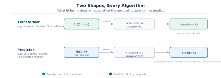
That two-step shape, learn parameters with fit, apply them with transform, is what scikit-learn calls a Transformer. It never sees a target value, only the columns it’s adjusting.
A model that predicts something works differently: it still has a fit step, but this time it’s learning a mapping from features to a known answer, and instead of transform it exposes predict.
demo_y: np.ndarray = np.array([1.0, 2.0, 3.0])
demo_lr: LinearRegression = LinearRegression()
demo_lr.fit(demo_x, demo_y)
demo_pred: np.ndarray = demo_lr.predict(new_point)
logger.info(f"Predicted y: {demo_pred}")
Key Concept: Transformer and Predictor
A Transformer has fit and transform. It learns something about the data’s shape, a mean, a scale, a set of categories, and never touches a target. A Predictor has fit(X, y) and predict(X). It learns a mapping to a known answer. StandardScaler, OneHotEncoder, and every other preprocessing step you meet in this book are Transformers. LinearRegression, LogisticRegression, and every model that follows are Predictors. Chapter 32’s Pipeline exists because a real project chains several of the first into exactly one of the second, and having a name for each half is what makes that chain readable.
3. Selecting and scaling features, before fitting anything real
Six interpretable columns, kept deliberately small so the mechanics stay visible: how far ahead someone booked, how many nights of each kind, how many adults, prior cancellations, and post-booking changes. Chapter 32 grows this into a full mixed feature set once the pattern here is solid.
FEATURES: list[str] = [
    "lead_time",
    "stays_in_weekend_nights",
    "stays_in_week_nights",
    "adults",
    "previous_cancellations",
    "booking_changes",
]
X: np.ndarray = df[FEATURES].to_numpy(dtype=float)
y_reg: np.ndarray = df[TARGET_REG].to_numpy(dtype=float)
y_clf: np.ndarray = df[TARGET_CLF].to_numpy(dtype=int)
logger.info(f"X: {X.shape}  y_reg: {y_reg.shape}  y_clf: {y_clf.shape}")
lead_time runs into the hundreds of days, adults rarely exceeds four. A model that updates its parameters by gradient, or measures distance between points, treats a feature with a bigger numeric range as more important by default, regardless of what it actually measures. Scaling puts every feature on the same footing before that happens.
Here’s the part that’s easy to get backwards: the scaler itself has to learn its mean and spread from training data only. Fit it on the full dataset before splitting, and the test set has quietly leaked its own distribution into the very transformation meant to be evaluated against it. The result looks like a working model and tells you nothing about how it performs on data it hasn’t seen.
for i, feat in enumerate(FEATURES):
    logger.info(f"  {feat:<30} min={X[:, i].min():>7.1f}  max={X[:, i].max():>7.1f}")
Split first, before the scaler learns anything:
X_tr, X_te, y_tr, y_te = train_test_split(X, y_reg, test_size=0.2, random_state=42)
logger.info(f"Train: {X_tr.shape}  Test: {X_te.shape}")
With the split done, fit the scaler on the training portion only:
scaler: StandardScaler = StandardScaler()
scaler.fit(X_tr)
logger.info(f"Learned means:  {scaler.mean_.round(2)}")
logger.info(f"Learned stds:   {scaler.scale_.round(2)}")
The same fitted scaler now applies to both sets. Same parameters, different input:
X_train_s: np.ndarray = scaler.transform(X_tr)
X_test_s: np.ndarray = scaler.transform(X_te)
for i, feat in enumerate(FEATURES):
    logger.info(f"  {feat:<30} min={X_train_s[:, i].min():>6.2f}  max={X_train_s[:, i].max():>6.2f}")
StandardScaler centres on the mean. MinMaxScaler squeezes everything into [0, 1] instead, useful for algorithms that expect bounded input, like a neural network’s first layer:
mms: MinMaxScaler = MinMaxScaler()
mms.fit(X_tr)
X_mm: np.ndarray = mms.transform(X_tr)
for i, feat in enumerate(FEATURES):
    logger.info(f"  {feat:<30} min={X_mm[:, i].min():.2f}  max={X_mm[:, i].max():.2f}")
Common Mistake: fitting the scaler before the split
# Wrong: the scaler sees every row, including the ones about to become test data
X_scaled = StandardScaler().fit_transform(X)
X_train_s, X_test_s = X_scaled[:n_train], X_scaled[n_train:]

# Correct: split first, fit on training rows only
X_tr, X_te, y_tr, y_te = train_test_split(X, y)
sc = StandardScaler().fit(X_tr)
X_train_s = sc.transform(X_tr)
X_test_s = sc.transform(X_te)
The wrong version still runs. It still produces a number. That number is just measuring something other than what it claims to.
Activity 2: RobustScaler
Fit a
Fit a
RobustScaler on X_tr (it centres on the median and scales by interquartile range instead of mean and standard deviation, so outliers pull it around less). Compare the scaled ranges against StandardScaler’s above.
from sklearn.preprocessing import RobustScaler
# your code here
Which feature moves the most compared to StandardScaler, and does that match which one had the widest raw range back in the first cell of this section?
4. Establishing baselines before anything smarter
Before any real model gets a turn, ask what the dumbest possible answer would score. DummyRegressor always predicts the training mean. DummyClassifier always predicts the training set’s most common class. Neither one learns anything about the six features you just scaled, and that’s the point: whatever a real model scores, it has to beat this first.
dummy_reg: DummyRegressor = DummyRegressor(strategy="mean")
dummy_reg.fit(X_train_s, y_tr)
dummy_pred: np.ndarray = dummy_reg.predict(X_test_s)
dummy_mae: float = mean_absolute_error(y_te, dummy_pred)
dummy_const: float = float(dummy_reg.constant_.flat[0])
logger.info(f"Dummy always predicts: {dummy_const:.2f} euros")
logger.info(f"Dummy MAE: {dummy_mae:.2f}")
€103.55 for every single booking, off by €35.66 on average. That’s the number Section 5’s model has to beat, and by how much determines whether the six features are worth anything at all.
Classification needs its own split, stratified so the 37% cancellation rate holds in both halves rather than drifting by chance:
Xc_tr, Xc_te, yc_tr, yc_te = train_test_split(X, y_clf, test_size=0.2, random_state=42, stratify=y_clf)
sc_clf: StandardScaler = StandardScaler()
Xc_train_s: np.ndarray = sc_clf.fit_transform(Xc_tr)
Xc_test_s: np.ndarray = sc_clf.transform(Xc_te)
logger.info(f"Train cancel rate: {yc_tr.mean():.2%}  Test cancel rate: {yc_te.mean():.2%}")
The classifier’s dummy baseline works the same way:
dummy_clf: DummyClassifier = DummyClassifier(strategy="most_frequent")
dummy_clf.fit(Xc_train_s, yc_tr)
dummy_clf_pred: np.ndarray = dummy_clf.predict(Xc_test_s)
dummy_f1: float = f1_score(yc_te, dummy_clf_pred, zero_division=0)
majority_class: int = int(dummy_clf.classes_[np.argmax(dummy_clf.class_prior_)])
logger.info(f"Dummy always predicts class: {majority_class}")
logger.info(f"Dummy F1: {dummy_f1:.3f}")
Zero. Not a low score, zero: predicting “not cancelled” for every booking gets roughly 63% of predictions right, since that’s the class majority, but it never once identifies an actual cancellation, and F1 punishes that completely. A model judged on plain accuracy could hide behind that same 63% and look almost as good as doing nothing. This is exactly why Chapter 30 picked F1 over accuracy for imbalanced problems: accuracy would have called this dummy baseline a decent model.
5. Linear models: a first real attempt
LinearRegression for ADR, LogisticRegression for cancellation, the two simplest Predictors that can actually learn from the six features instead of ignoring them. One evaluation helper covers every regression comparison the rest of this notebook makes:
def evaluate_regressor(model: Any, X_eval: np.ndarray, y_eval: np.ndarray, name: str) -> dict[str, Any]:
    """Return MAE, RMSE, and R2 for a fitted regression model."""
    preds: np.ndarray = model.predict(X_eval)
    return {
        "Model": name,
        "MAE": float(mean_absolute_error(y_eval, preds)),
        "RMSE": float(mean_squared_error(y_eval, preds) ** 0.5),
        "R2": float(r2_score(y_eval, preds)),
    }
With that ready, fit the model it will judge:
lin_reg: LinearRegression = LinearRegression()
lin_reg.fit(X_train_s, y_tr)
logger.success("LinearRegression fitted")
Compare it against the baseline:
reg_results: pd.DataFrame = pd.DataFrame(
    [
        evaluate_regressor(dummy_reg, X_test_s, y_te, "DummyRegressor (mean)"),
        evaluate_regressor(lin_reg, X_test_s, y_te, "LinearRegression"),
    ]
)
metrics_report(
    reg_results,
    metrics=["MAE", "RMSE", "R2"],
    minimize_cols=["MAE", "RMSE"],
    maximize_cols=["R2"],
    title="Regression performance: ADR prediction",
    subtitle="Test set | Hotel Booking Demand dataset",
)| Regression performance: ADR prediction | |||
| Test set | Hotel Booking Demand dataset | |||
| Model | MAE | RMSE | R2 |
|---|---|---|---|
| DummyRegressor (mean) | 35.665 | 46.904 | −0.000 |
| LinearRegression | 33.800 | 44.425 | 0.103 |
| DS-MLOps Path | |||
€33.80 MAE against the dummy’s €35.66: a real improvement, but a small one, and R2 of 0.10 says these six features explain barely a tenth of why one booking costs more than another. That’s not a failed model, it’s an honest one: lead time, party size, and a handful of stay-length counts were never going to price a hotel room on their own, room type and season do most of that work, and neither is in FEATURES yet. The coefficients show which of the six is carrying what little signal there is:
coef_df: pd.DataFrame = (
    pd.DataFrame({"feature": FEATURES, "coefficient": lin_reg.coef_})
    .sort_values("coefficient", key=abs, ascending=False)
    .reset_index(drop=True)
)
themed_gt(GT(coef_df), n_rows=len(coef_df)).tab_header(
    title=gt_md("**LinearRegression coefficients**"),
    subtitle="Standardised features: magnitude reflects relative importance",
)| LinearRegression coefficients | |
| Standardised features: magnitude reflects relative importance | |
| feature | coefficient |
|---|---|
| adults | 14.010392473075402 |
| lead_time | -5.999478571038943 |
| previous_cancellations | -2.685241761638044 |
| booking_changes | 2.321032378136231 |
| stays_in_week_nights | 1.4716065708455348 |
| stays_in_weekend_nights | -0.17308457446668957 |
coef_plot: pd.DataFrame = coef_df.assign(
    color=lambda d: d["coefficient"].apply(lambda v: "positive" if v >= 0 else "negative")
)
(
    ggplot(coef_plot, aes(x=as_discrete("feature", order_by="coefficient", order=1), y="coefficient", fill="color"))
    + geom_bar(stat="identity", alpha=0.85)
    + scale_fill_manual(values={"positive": INFO, "negative": DANGER})
    + labs(
        title="LinearRegression coefficients",
        subtitle="Standardised features: positive raises ADR, negative lowers it",
        x="",
        y="Coefficient",
    )
    + modern_theme(x_axis_angle=30, legend_pos="none")
)
More adults pushes the price up (+14.01, the largest effect by far, a bigger room for a bigger party), and a longer lead time pulls it down (-6.00): book far enough ahead and you tend to catch an early, lower rate. A residual plot checks whether the model is missing something systematic, or just noisy in a way six weak features would predict:
y_pred_lin: np.ndarray = lin_reg.predict(X_test_s)
resid_df: pd.DataFrame = pd.DataFrame({"predicted": y_pred_lin, "residual": y_te - y_pred_lin})
(
    ggplot(resid_df, aes(x="predicted", y="residual"))
    + geom_point(color=INFO, alpha=0.12, size=1)
    + geom_hline(yintercept=0, color=DANGER, linetype="dashed", size=1)
    + labs(
        title="Residuals vs predicted ADR",
        subtitle="Random scatter around zero: no systematic bias, just weak signal",
        x="Predicted ADR (euros)",
        y="Residual (actual minus predicted)",
    )
    + modern_theme(grid=True)
)
No curve, no funnel, just a wide, roughly even scatter. The model isn’t systematically wrong about any particular price range, it’s just working with features that don’t carry enough information to narrow the scatter further. That’s a feature problem, not a modelling-technique problem, the same lesson Case Study 1 makes with real dollar figures on a different dataset.
Cancellation gets LogisticRegression, with one adjustment LinearRegression didn’t need: class_weight="balanced" reweights the loss so the majority class (kept bookings) can’t dominate the way it did for the dummy baseline. Without it, a model minimising raw error learns to predict “not cancelled” almost everywhere, for the same reason the dummy classifier scored zero F1.
log_reg: LogisticRegression = LogisticRegression(class_weight="balanced", max_iter=1000, random_state=42)
log_reg.fit(Xc_train_s, yc_tr)
logger.success("LogisticRegression fitted")
See how it actually performs:
yc_pred: np.ndarray = log_reg.predict(Xc_test_s)
report: str = classification_report(yc_te, yc_pred, target_names=["Kept", "Cancelled"])
logger.info("\n" + report)
0.55 F1 on the cancelled class, against the dummy’s 0.0. Recall of 0.54 means it catches just over half of the bookings that will actually cancel, precision of 0.56 means just over half of what it flags really does cancel. Not good enough to automate a decision on yet, but a real, measurable signal where the baseline had none.
Activity 3: Ridge vs LinearRegression
Ridge adds an L2 penalty that shrinks coefficients toward zero, which can reduce overfitting on noisier data.
from sklearn.linear_model import Ridge
ridge = Ridge(alpha=1.0)
ridge.fit(X_train_s, y_tr)
# compare evaluate_regressor(ridge, ...) against lin_reg
Given R2 was already only 0.10 with plain LinearRegression, do you expect Ridge to move the number much? Check whether it does.
6. Cross-validation: trusting the number more
One train/test split gives one number, and that number carries whatever noise happened to land in that particular 20%. Cross-validation rotates the held-out portion across five folds, in turn: each fold takes a turn as validation while the other four train, producing five scores instead of one, and the mean plus standard deviation of those five is a far steadier estimate than any single split.
Wrapping the scaler and model in a Pipeline first isn’t optional here. Pass the model alone to cross_val_score and every fold’s “training” score is still computed against a scaler fitted on all five folds at once, leaking exactly the way Section 3’s Common Mistake did. Pipeline re-fits the scaler inside each fold automatically, Chapter 32 is built entirely around making that guarantee explicit.
reg_pipe: Pipeline = Pipeline([("scaler", StandardScaler()), ("model", LinearRegression())])
kf: KFold = KFold(n_splits=5, shuffle=True, random_state=42)
cv_reg: np.ndarray = cross_val_score(reg_pipe, X_tr, y_tr, cv=kf, scoring="neg_mean_absolute_error")
logger.info(f"CV MAE per fold: {(-cv_reg).round(2)}")
logger.info(f"Mean +/- std: {-cv_reg.mean():.2f} +/- {cv_reg.std():.2f}")
€33.57 ± €0.14: five folds within fifteen cents of each other. That tight a spread says the single-split MAE from Section 5 (€33.80) wasn’t a lucky or unlucky split, it’s a stable, reproducible number. Classification needs StratifiedKFold instead of plain KFold, for the same reason the earlier split used stratify=y_clf: with only 37% of bookings cancelling, an unlucky fold boundary could hand one fold almost no cancellations at all, and a metric like F1 becomes meaningless on a fold with too few positive examples to compute it from.
clf_pipe: Pipeline = Pipeline(
    [
        ("scaler", StandardScaler()),
        ("model", LogisticRegression(class_weight="balanced", max_iter=1000, random_state=42)),
    ]
)
skf: StratifiedKFold = StratifiedKFold(n_splits=5, shuffle=True, random_state=42)
cv_clf: np.ndarray = cross_val_score(clf_pipe, Xc_tr, yc_tr, cv=skf, scoring="f1")
logger.info(f"CV F1 per fold: {cv_clf.round(3)}")
logger.info(f"Mean +/- std: {cv_clf.mean():.3f} +/- {cv_clf.std():.3f}")
0.554 ± 0.003, just as tight. Both cross-validated numbers land almost exactly where the single split already put them, which is itself the useful finding: on a dataset this size, a single stratified split was already a trustworthy estimate. That won’t hold on every dataset this book uses, which is exactly why the check is worth running rather than assuming.
7. Learning curves: more data, or a better model?
Section 5 left an open question: is 0.10 R2 a ceiling this feature set can’t get past, or would a bigger training set push it higher? A learning curve answers this by refitting the pipeline at increasing training sizes and watching what happens to the gap between training and validation error.
train_sizes: np.ndarray
train_lc_scores: np.ndarray
val_lc_scores: np.ndarray
train_sizes, train_lc_scores, val_lc_scores = learning_curve(
    reg_pipe,
    X_tr,
    y_tr,
    train_sizes=np.linspace(0.1, 1.0, 8),
    cv=KFold(n_splits=5, shuffle=True, random_state=42),
    scoring="neg_mean_absolute_error",
    n_jobs=-1,
)
train_sizes
array([ 7515, 17178, 26840, 36503, 46166, 55828, 65491, 75154])lc_df: pd.DataFrame = pd.DataFrame(
{
"n": np.tile(train_sizes, 2),
"score": np.concatenate([-train_lc_scores.mean(1), -val_lc_scores.mean(1)]),
"err": np.concatenate([train_lc_scores.std(1), val_lc_scores.std(1)]),
"split": ["Train"] * len(train_sizes) + ["Validation"] * len(train_sizes),
}
).assign(ymin=lambda d: d["score"] - d["err"], ymax=lambda d: d["score"] + d["err"])
(
ggplot(lc_df, aes(x="n", y="score", color="split", fill="split"))
+ geom_line(size=1.2)
+ geom_ribbon(aes(ymin="ymin", ymax="ymax"), alpha=0.15, color=None)
+ scale_color_manual(values={"Train": INFO, "Validation": WARNING})
+ scale_fill_manual(values={"Train": INFO, "Validation": WARNING})
+ labs(
title="Learning curve: LinearRegression on ADR",
subtitle="Flat from the smallest training size tested: a features problem, not a data problem",
x="Training set size",
y="MAE (lower is better)",
)
+ modern_theme(grid=True, legend_pos="bottom")
)Training and validation MAE sit within a few cents of each other at every size tested, including the smallest, 7,515 rows. There’s no gap to close: this isn’t a model straining against too little data, it’s a model that hit its ceiling almost immediately and stayed there while the training set grew tenfold. More bookings would not move this number. A feature that actually explains price, room type, season, how far in advance the rate was locked in, would. That’s the same conclusion Section 5’s weak R2 already pointed to, confirmed a second way.
Activity 4: learning curve for LogisticRegression
Compute and plot a learning curve for clf_pipe using scoring=“f1” and StratifiedKFold in place of KFold. Does the cancellation classifier show the same flat, converged shape, or is there still a gap between train and validation that more data might close?
8. Saving what you built
A fitted model is only half of what production needs. Predict on raw, unscaled input with a model trained on scaled input and you get a number, just not a meaningful one, the model has no way to tell you it was handed the wrong kind of input. The scaler and the model have to travel together, saved as one bundle, not two files someone has to remember to load in the right order.
MODEL_DIR.mkdir(exist_ok=True)
model_path: Path = MODEL_DIR / "lin_reg_adr.joblib"
bundle: dict[str, Any] = {"scaler": scaler, "model": lin_reg, "features": FEATURES, "target": TARGET_REG}
joblib.dump(bundle, model_path)
logger.success(f"Bundle saved to {model_path}")
Reload it in a fresh call to confirm the bundle actually works end to end:
loaded: dict[str, Any] = joblib.load(model_path)
sample: np.ndarray = X_te[:1]
sample_scaled: np.ndarray = loaded["scaler"].transform(sample)
predicted: float = float(loaded["model"].predict(sample_scaled)[0])
actual: float = float(y_te[0])
logger.info(f"Predicted ADR: {predicted:.2f}  Actual ADR: {actual:.2f}")
Pro Tip: save the scaler inside the bundle, never separately
A model evaluated on unscaled inputs in production is one of the most common silent bugs in deployed ML systems: it doesn’t crash, it just predicts wrong, quietly, at whatever confidence it would have had on correctly scaled data. Bundling scaler and model as one object removes the chance to load one without the other.
Packaging the pattern for reuse
Split, scale, fit, evaluate, save: the same five steps ran twice in this chapter, once for ADR and once for cancellation, with only the model and the metric changing. Writing it once as a typed function isn’t just tidier, it’s the exact shape Chapter 32 inherits and formalises into a Pipeline object.
def train_and_evaluate(
    df: pd.DataFrame,
    features: list[str],
    target: str,
    task: str,
    out_dir: Path = Path("models"),
) -> dict[str, Any]:
    """Run the full train-evaluate-save workflow for one task."""
    X_all: np.ndarray = df[features].to_numpy(dtype=float)
    y_all: np.ndarray = df[target].to_numpy()

    stratify: np.ndarray | None = y_all if task == "classification" else None
    Xtr, Xte, ytr, yte = train_test_split(X_all, y_all, test_size=0.2, random_state=42, stratify=stratify)
    sc: StandardScaler = StandardScaler()
    Xtr_s: np.ndarray = sc.fit_transform(Xtr)
    Xte_s: np.ndarray = sc.transform(Xte)

    if task == "regression":
        model: Any = LinearRegression()
        baseline: Any = DummyRegressor(strategy="mean")
    else:
        model = LogisticRegression(class_weight="balanced", max_iter=1000, random_state=42)
        baseline = DummyClassifier(strategy="most_frequent")

    baseline.fit(Xtr_s, ytr)
    model.fit(Xtr_s, ytr)

    if task == "regression":
        m: dict[str, float] = {
            "baseline_mae": float(mean_absolute_error(yte, baseline.predict(Xte_s))),
            "model_mae": float(mean_absolute_error(yte, model.predict(Xte_s))),
            "model_r2": float(r2_score(yte, model.predict(Xte_s))),
        }
    else:
        m = {
            "baseline_f1": float(f1_score(yte, baseline.predict(Xte_s), zero_division=0)),
            "model_f1": float(f1_score(yte, model.predict(Xte_s))),
        }

    out_dir.mkdir(exist_ok=True)
    save_path: Path = out_dir / f"{target}.joblib"
    joblib.dump({"scaler": sc, "model": model, "features": features, "target": target}, save_path)
    logger.success(f"Saved {task} bundle for '{target}' to {save_path}")
    logger.info(f"Metrics: {m}")
    return {"model": model, "scaler": sc, "metrics": m}
reg_result: dict[str, Any] = train_and_evaluate(df, FEATURES, TARGET_REG, task="regression", out_dir=MODEL_DIR)clf_result: dict[str, Any] = train_and_evaluate(df, FEATURES, TARGET_CLF, task="classification", out_dir=MODEL_DIR)Neither model is ready to run a hotel on. The regression model can’t yet explain the price a room should carry, only rank it weakly against six thin proxies, missing room type and season entirely. The classifier catches barely half of the bookings that will cancel. Both are honest first attempts, and both point at the same next move: better features, not a fancier algorithm on the same six columns, the exact lesson Case Study 1 proves with a dollar figure attached later in this book.
What’s solid is the shape: a Transformer and a Predictor, fit only on training data, evaluated against a baseline, cross-validated instead of trusted on one split, and saved as a single bundle. Six fit calls ran across this chapter, scaler and model, twice over, plus a third pair inside the capstone function. Six places a leak or a mismatched scaler could have crept in. Chapter 32 collapses all of it into one object that makes those six calls impossible to get out of order.
Further reading
- Scikit-learn user guide
- Geron, A. (2022), Hands-On Machine Learning, Ch 2-4
- Antonio et al. (2019), Hotel booking demand datasets, Data in Brief
Summary
| Concept | Key rule |
|---|---|
| Transformer | Has fit and transform; never sees a target; e.g. StandardScaler, OneHotEncoder |
| Predictor | Has fit(X, y) and predict(X); learns a mapping to a known answer |
| Split before scaling | Fit a scaler (or any transformer) on training data only; fitting before the split leaks the test distribution into the transformation |
| Baseline first | DummyRegressor/DummyClassifier show what “no model” scores; a real model has to beat that number, not just produce one |
class_weight="balanced" |
Reweights the loss so a majority class can’t win by default; without it, an imbalanced target gets predicted as one class almost everywhere |
| Cross-validation | Rotates the held-out fold across five splits; mean +/- std is a steadier estimate than any single split’s score |
| Learning curve | A flat train/validation gap at every size says more data won’t help; the ceiling is the features, not the sample size |
| Model bundle | Save the scaler and the model together; a model scored on unscaled input predicts wrong without ever raising an error |
Next: Chapter 32 wraps every one of these separate fit calls into a single Pipeline object, and grows the six-feature model here into fourteen columns across two treatments.