You have built the chart. The axes are labelled, the data is correct. You export it and paste it into the slide deck. Ten minutes later someone asks: “What am I supposed to take from this?” The chart was not wrong. It was just not a story.
Chapters 14 and 15 taught you the mechanics: matplotlib’s object model, lets-plot’s grammar of graphics. This notebook is about judgment: which chart to pick, what ink to cut, how your eye is deceived by common tricks, and how to apply a house style so every chart you publish looks like it belongs to the same project. Chapter 17 puts every one of these judgment calls to work on a single real case, start to finish.
Choose a chart type based on the question, not habit
Sec. 1
2
Apply Gestalt principles to explain why grouped charts work
Sec. 2
3
Recognise and avoid the most common ways charts mislead
Sec. 3
4
Decide when a table communicates better than a chart
Sec. 4
5
Apply ark.plot’s house theme to matplotlib and lets-plot charts
Sec. 5
6
Identify preattentive attributes and use them deliberately
Sec. 6
7
Add annotations that carry the chart’s narrative
Sec. 7
8
Explain why summary statistics alone are never sufficient (Datasaurus)
Sec. 8
9
Produce one polished, captioned chart from a messy dataset
Capstone
1. Picking the Right Chart, and Cutting What Does Not Help
The most common visualisation mistake isn’t a styling problem, it’s a selection problem: building a chart type out of habit instead of asking what question it needs to answer. A pie chart can’t answer “which course improved the most,” because comparing angles is something people are measurably worse at than comparing positions along a shared axis. That isn’t opinion, it’s the finding of a well-known study by Cleveland and McGill (1984) ranking how accurately people read different visual encodings: position along a common scale first, then length, then angle, then area, with colour saturation last.
import numpy as npimport pandas as pd# Full platform export, used directly wherever a chart doesn't need a fixed category countdf7 = pd.read_csv("data/university_analytics.csv")# Same three-course, three-Fall-cohort slice as Chapters 14 and 15, so every# chart in this notebook is comparing the same students_courses = ["Machine Learning", "Data Structures", "Python Programming"]_semesters = ["Fall 2022", "Fall 2023", "Fall 2024"]results = df7[df7["course"].isin(_courses) & df7["semester"].isin(_semesters)].copy()results.head()
student_id
cohort
program
gender
region
guardian
has_internet
course_id
course
semester
enrollment_date
study_hours
attendance_pct
midterm_score
final_score
project_score
final_grade
passed
0
S0001
2023
Information Technology
F
South
Father
True
C01
Python Programming
Fall 2023
2023-09-04
10.8
88.6
49.9
58.2
61.6
C
True
2
S0001
2023
Information Technology
F
South
Father
True
C03
Data Structures
Fall 2023
2023-09-04
23.6
71.5
54.1
60.9
79.8
C
True
4
S0001
2023
Information Technology
F
South
Father
True
C05
Machine Learning
Fall 2023
2023-09-04
16.2
63.2
48.4
54.2
51.8
D
True
6
S0002
2023
Data Science
M
West
Mother
True
C01
Python Programming
Fall 2023
2023-09-04
17.4
67.0
93.6
60.5
67.0
B
True
8
S0002
2023
Data Science
M
West
Mother
True
C03
Data Structures
Fall 2023
2023-09-04
30.4
84.9
67.4
93.5
70.6
B
True
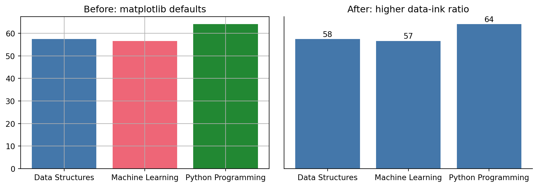
Data-ink ratio, a term from Edward Tufte’s The Visual Display of Quantitative Information, is the proportion of a chart’s ink that represents actual data, as opposed to gridlines, borders, redundant legends, and other decoration. Maximising it doesn’t mean a bare chart, it means every mark earns its place. Alberto Cairo calls this “functional art”: a chart still has to be engaging, it just can’t be engaging instead of being clear. Compare matplotlib’s defaults to a version with the same data and nothing extra:
import matplotlib.pyplot as pltcourse_means = results.groupby("course")["final_score"].mean()fig, axes = plt.subplots(1, 2, figsize=(10, 3.5))# Left: matplotlib defaults. Box on all four sides, both gridlines, a# legend the bar colours already make redundant since each bar has its# own label directly underneath it.axes[0].bar(course_means.index, course_means.values, color=["#4477AA", "#EE6677", "#228833"])axes[0].set_title("Before: matplotlib defaults")axes[0].grid(True)# Right: same data, decluttered. No top/right spines, no gridlines, the# value printed directly on each bar instead of relying on the y-axis.axes[1].bar(course_means.index, course_means.values, color="#4477AA")axes[1].spines["top"].set_visible(False)axes[1].spines["right"].set_visible(False)axes[1].set_yticks([])for i, value inenumerate(course_means.values): axes[1].text(i, value +1, f"{value:.0f}", ha="center")axes[1].set_title("After: higher data-ink ratio")fig.tight_layout()
Key Concept: Data-ink ratio
Every gridline, border, and redundant legend entry competes with your data for the reader’s attention. The right-hand chart above removes the y-axis entirely (the labelled bars make it redundant) and the top/right spines, and prints each value once, directly on its bar, instead of forcing the reader to trace a line back to an axis. Decluttering isn’t about making a chart sparse for its own sake, it’s about removing anything that doesn’t carry information.
One message per chart is the last principle worth internalising before the chart-lie gallery in Section 2: a chart that tries to answer three questions at once usually answers none of them clearly. If you find yourself adding a third colour dimension, a secondary y-axis, and a trend line to the same chart, that is a sign you need two charts, not one crowded one.
Activity 1 - Cut the Ink
Apply the data-ink ratio principle to the comparison chart from this section.
1. Copy the fig, axes = plt.subplots(1, 2) comparison code from above into a new cell. 2. On the ‘before’ panel, add two extra elements that increase ink without adding information: ax.grid(True) and ax.set_facecolor(‘#F0F0F0’). 3. On the ‘after’ panel, remove every element you can: spines, tick labels, background: keep only what is needed to read the values. 4. Add a markdown cell: ‘I removed X because…’ for each removed element.
Expected: the ‘after’ panel communicates the same data with fewer marks.
2. Gestalt Principles: Why Grouped Charts Work
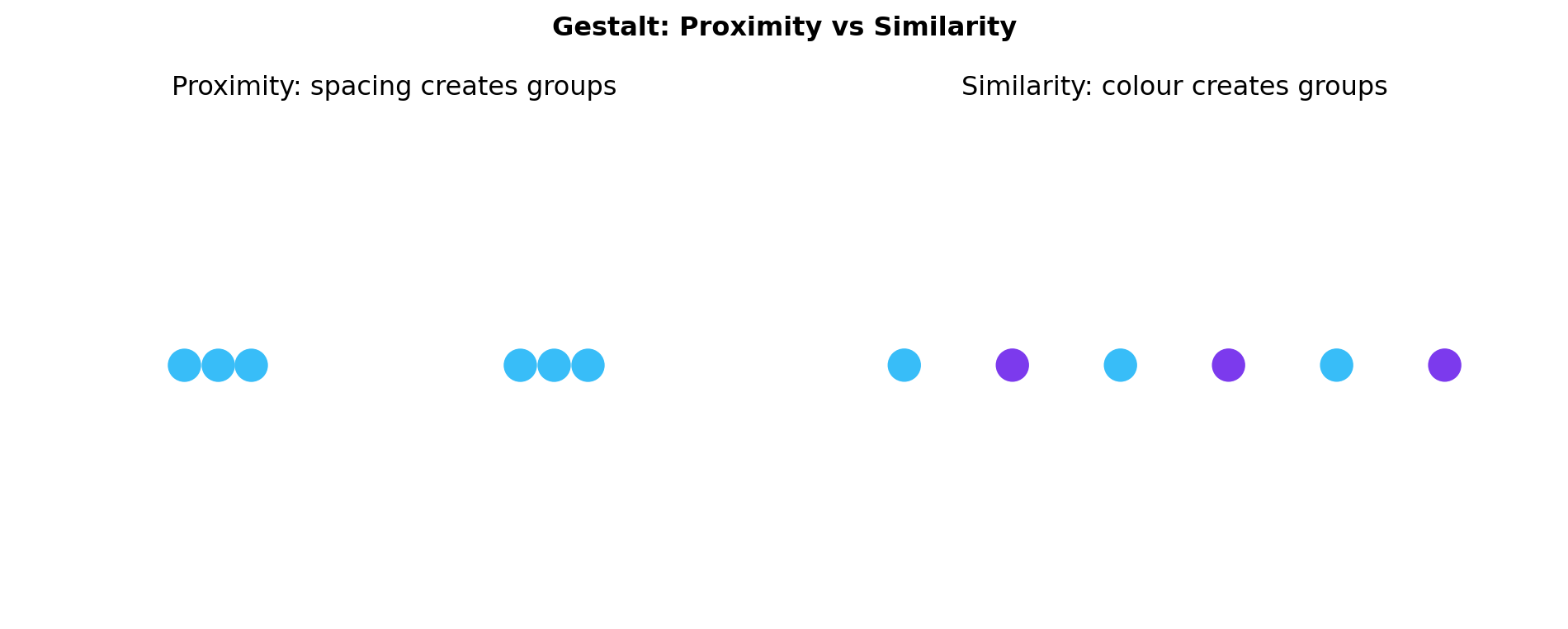
Preattentive attributes tell you what stands out before conscious attention. Gestalt principles tell you how the brain groups what it sees. The two work together: colour creates salience (preattentive); proximity creates grouping (Gestalt). Four principles appear everywhere in DS charts.
Key Concept: Four Gestalt Principles in Chart Design
The four Gestalt principles used in chart design: (1) Proximity: elements near each other are perceived as a group: this is why grouped bars and facets work; (2) Similarity: elements sharing colour, shape, or size seem to belong together; (3) Enclosure: a box, border, or shaded region creates a visual group; (4) Continuity: the eye follows a smooth path: this is why line charts work for time series but not categorical comparisons.
Activity 2 - Proximity Without a Legend
Use layout alone to group related series without adding a legend.
1. Create a fig, axes = plt.subplots(1, 2, figsize=(9, 3.5), sharey=True). 2. On the left panel plot Maths and Statistics scores as two overlapping histograms with alpha=0.6 in brand colours. 3. On the right panel plot Programming and Data Science the same way. 4. Add a title to each panel that says what it shows: no legend.
Expected: proximity (left vs right) groups the courses; the title replaces the legend.
3. Common Chart Lies
None of the charts below contain incorrect numbers. Each one is drawn in a way that makes the reader’s brain compute the wrong conclusion from correct data. Recognising these on sight, in your own draft charts, is the actual skill.
Key Concept: A misleading chart shows correct numbers in a deceptive frame
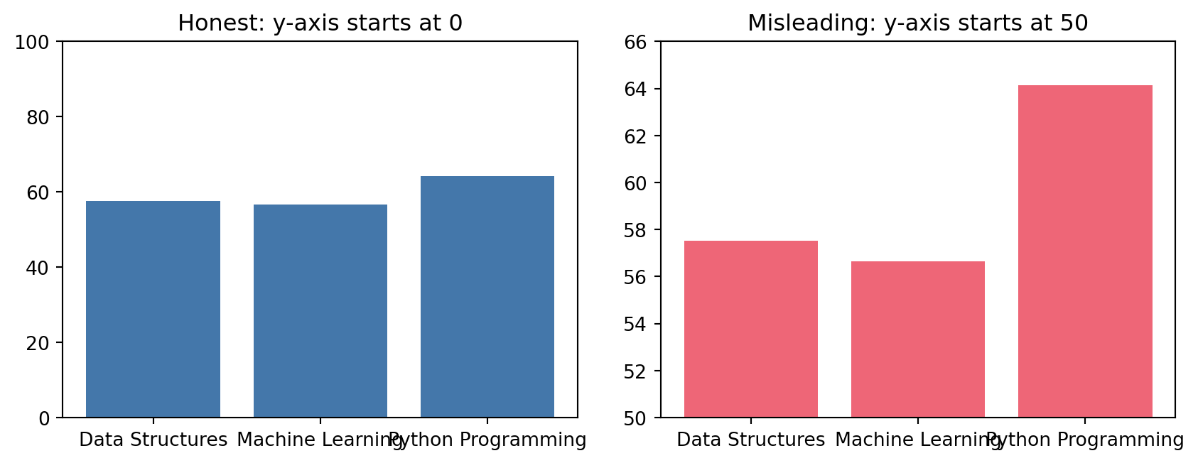
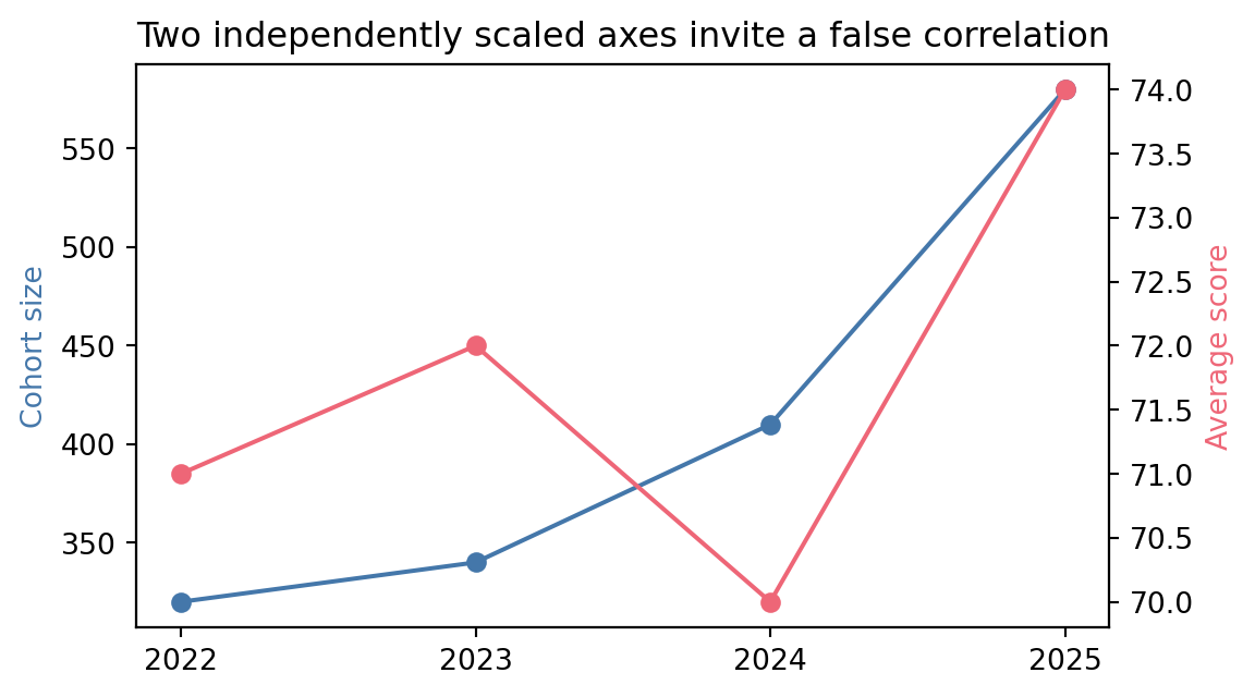
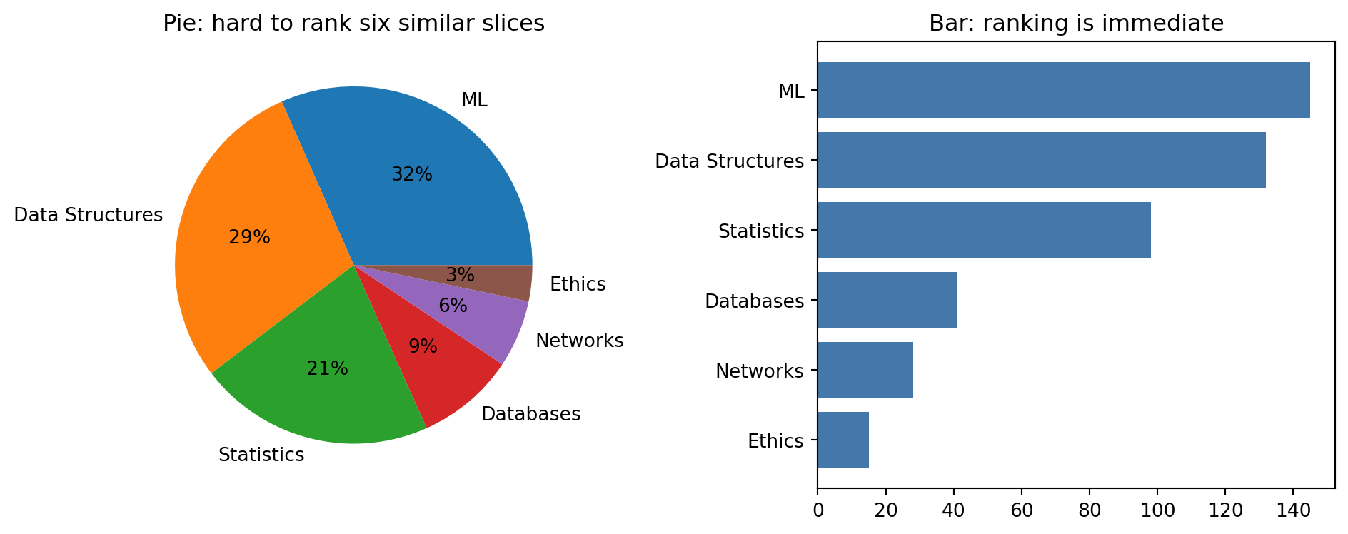
Truncating the y-axis at a non-zero value makes small differences look large. A dual y-axis on the same plot invites the reader to see causation in coincidence. A pie chart with six slices is almost impossible to read because humans compare angles poorly. None of these charts lie about the numbers: they lie about what the numbers mean.
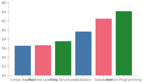
The two charts above show the exact same three numbers. The right-hand one starts its y-axis at 50 instead of 0, which makes a 7-point difference between courses look like one course scores roughly twice as high as another. Bar charts in particular must start at zero, because the reader judges bar height (and therefore a ratio) automatically. Line charts can sometimes justify a non-zero baseline if it’s labelled clearly, bars almost never can.
Cohort size and average score both happen to rise together in this chart, but each axis was scaled independently to make the two lines fit nicely, which is exactly what makes dual axes dangerous: you can almost always pick scales that make two unrelated series appear to move together. If two series genuinely need comparing, plot their percent change from a common baseline on one shared axis instead, or use two separate charts stacked vertically with the same x-axis.
enrollment = pd.Series( {"ML": 145, "Data Structures": 132, "Statistics": 98, "Databases": 41, "Networks": 28, "Ethics": 15})fig, axes = plt.subplots(1, 2, figsize=(10, 4))axes[0].pie(enrollment.values, labels=enrollment.index, autopct="%1.0f%%")axes[0].set_title("Pie: hard to rank six similar slices")axes[1].barh(enrollment.index[::-1], enrollment.values[::-1], color="#4477AA")axes[1].set_title("Bar: ranking is immediate")fig.tight_layout()
Common Mistake: Too many pie slices
Six categories is already past where a pie chart works: Ethics and Networks are visibly different bars, but as pie slices they are nearly impossible to rank by eye, exactly the angle-judgment weakness Cleveland and McGill measured. A horizontal bar chart, sorted by value, answers “which course has the most enrollment” instantly. Reserve pie charts for two or three categories where one slice is clearly dominant, and prefer a bar chart almost everywhere else.
Activity 3 - Fix the Truncated Y-Axis
Spot and correct a chart lie in this section.
1. Re-run the truncated y-axis bar chart from this section. 2. Add axes[0].set_ylim(0, None) to start the scale at zero. 3. In a markdown cell below, describe in one sentence how the story changes when the axis starts at zero.
Expected: the differences between courses look smaller; the story is more honest.
4. When a Table Beats a Chart
A chart is for spotting a pattern at a glance. A table is for looking up an exact number, or comparing many numbers a reader needs to cite precisely, such as a results appendix someone will quote in a report. This project’s ark.plot.gt_style module wraps great_tables with the same brand colours used everywhere else, so a results table looks like it belongs in the same document as the chart next to it:
Key Concept: Use a chart for patterns, a table for lookups
A chart answers: ‘is there a trend, a cluster, an outlier?’ A table answers: ‘what was the exact value for X in period Y?’ If your reader needs to look up a specific number, a table is faster. If your reader needs to see a shape across many values at once, a chart is faster. Showing both for the same data wastes space and splits attention.
from great_tables import GT, md as gt_mdfrom ark.plot.gt_style import themed_gtsummary = results.groupby("course")["final_score"].agg(mean="mean", std="std", n="count").round(1).reset_index()table = themed_gt( GT(summary) .tab_header(title=gt_md("**Final Score Summary**"), subtitle="Mean, spread, and sample size per course") .cols_label(course="Course", mean="Mean", std="Std. Dev.", n="N"), n_rows=len(summary),)table
Final Score Summary
Mean, spread, and sample size per course
Course
Mean
Std. Dev.
N
Data Structures
57.5
14.4
400
Machine Learning
56.6
15.3
400
Python Programming
64.1
15.4
400
Pro Tip: Pair a chart with a table, don’t choose between them
A results section in a report often wants both: the histogram from Chapter 14 to show the shape of the distribution, and a table like the one above to give the exact numbers someone will want to quote. Neither replaces the other.
Activity 4 - Chart vs Table Decision
Decide which form is right for the question.
1. Create the summary table from this section (mean, std, n per course). 2. Also create a line chart of mean final score by course using matplotlib. 3. In a markdown cell, answer: a department head wants to compare pass rates at a glance: which do you show and why? 4. Now answer: a student wants to know their course’s exact mean: which do you show and why?
Expected: different questions, different answers.
5. From Default to Branded
Chapters 14 and 15 used each library’s own defaults on purpose, so the charts in those notebooks teach the mechanics without a styling layer in the way. This project’s ark.plot module exists precisely so you don’t have to restate the same colours, fonts, and spacing on every single chart by hand. Compare a lets-plot chart with and without it:
Apply the same transformation to the full dataset:
from lets_plot import labs, scale_fill_manualfrom ark.plot.theme import modern_theme, pro_colorsbranded_chart = ( ggplot(results, aes(x="final_score", fill="course"))+ geom_histogram(bins=20, alpha=0.85)+ scale_fill_manual(values=pro_colors)+ labs( title="Final score distribution by course", x="Final score (0-100)", y="Number of students", fill="Course", )+ modern_theme(grid=True))branded_chart + ggsize(450, 300)
modern_theme() is one more + layer, exactly like every geom_*() in Chapter 15. scale_fill_manual(values=pro_colors) pins each course to the brand palette, and labs() replaces the auto-generated column names with reader-facing text. gggrid() puts both charts side by side in one output, which is the cleanest way to show a before/after comparison in a single cell:
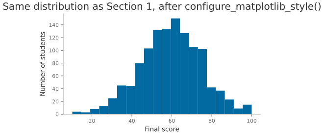
The matplotlib equivalent, ark.plot.matplot_theme.configure_matplotlib_style(), works differently: it updates matplotlib’s global rcParams, so it applies to every chart drawn after you call it, not just one. That is the right trade-off for a notebook or script that draws many charts you want to look consistent, at the cost of not being able to mix styled and unstyled charts in the same figure:
from ark.plot.matplot_theme import configure_matplotlib_styleconfigure_matplotlib_style(font_size=10, fig_width=5)fig, ax = plt.subplots()ax.hist(results["final_score"], bins=20)ax.set_xlabel("Final score")ax.set_ylabel("Number of students")ax.set_title("Same distribution as Section 1, after configure_matplotlib_style()");
Key Concept: House style is a default, not a style applied chart by chart
Calling configure_matplotlib_style() once at the top of a notebook applies the same font size, spine removal, and grid style to every subsequent matplotlib chart. Passing modern_theme() and a branded colour scale once defines the look for every lets-plot chart in the session. The goal is consistency across an entire report, not per-chart customisation.
Activity 5 - Brand a Boxplot
Rebuild Chapter 14’s seaborn boxplot of final_score by course, but after calling configure_matplotlib_style() from this section. No other code changes: the same sns.boxplot() call should now pick up the brand colour cycle automatically.
import seaborn as sns# TODO: boxplot of final_score by course, styled by the already-active house theme...
Ellipsis
Pro Tip: A house theme is a contract, not a one-off setting
The value of ark.plot isn’t any single colour choice, it’s that every chart in this project, in any notebook, in any report, reaches for the same module instead of redefining its own palette. When the brand colours change, they change in one file.
6. Preattentive Attributes: What the Brain Sees First
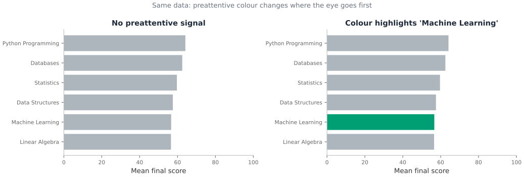
Before you consciously read a chart, your visual system has already processed certain features. These are called preattentive attributes: colour hue, luminance, shape, orientation, size, position, and enclosure. They register in under 250 milliseconds, before attention is directed.
The design implication is simple but easy to violate: use at most one preattentive attribute for emphasis per chart. Two or more compete for attention and cancel each other out.
Key Concept: Preattentive Attributes
Visual properties processed before conscious attention: colour hue, luminance, shape, orientation, size, position, and motion. The practical rule: encode at most one categorical dimension preattentively, and make sure it carries information, not decoration.
Reference: Ware, C. (2012). Information Visualization: Perception for Design, 3rd ed.
import matplotlib.pyplot as pltimport numpy as npimport pandas as pddf7 = pd.read_csv("data/university_analytics.csv")course_means = df7.groupby("course")["final_score"].mean().sort_values()# Left: every bar the same colour: no preattentive signal# Right: one bar highlighted with colour: attention goes there instantlyTARGET ="Machine Learning"fig, axes = plt.subplots(1, 2, figsize=(11, 3.8))for ax, use_highlight inzip(axes, [False, True], strict=False): colors = ( ["#009E73"if c == TARGET else"#ADB5BD"for c in course_means.index]if use_highlightelse ["#ADB5BD"] *len(course_means) ) ax.barh(course_means.index, course_means.values, color=colors) ax.set_xlabel("Mean final score") ax.spines[["top", "right"]].set_visible(False) ax.set_xlim(0, 100) title ="No preattentive signal"ifnot use_highlight elsef"Colour highlights {TARGET!r}" ax.set_title(title, fontsize=11, fontweight="bold", color="#1E293B")fig.suptitle("Same data: preattentive colour changes where the eye goes first", fontsize=10, color="#6B7280")fig.tight_layout()plt.show()
Activity 6 - Highlight by Region
Build a horizontal bar chart of mean midterm_score by region. Highlight the region with the highest mean in #0369A1 and colour every other bar #ADB5BD. Add a concise title stating which region leads.
region_means = df7.groupby("region")["midterm_score"].mean().sort_values()
# ... build the chart with one highlighted bar ...
# TODO: highlight the top-scoring region in the midterm score chart...
7. Annotation as Narrative
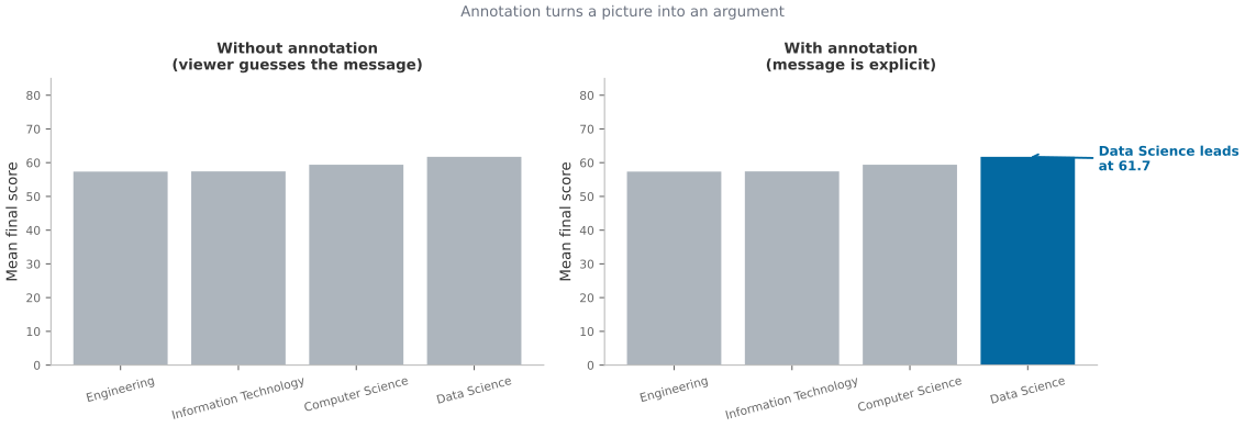
A chart without annotation forces viewers to form their own interpretation. Annotation is where the “so what?” lives: the one sentence that turns a picture into an argument.
Effective annotation does three things: 1. Points at the specific data feature that supports the message (arrow or callout). 2. States that feature in plain language, not chart jargon. 3. Uses restraint: one annotation per message, not one per data point.
Key Concept: Annotation as the “So What?”
Knaflic’s rule (2015): “the most important single thing you can do to improve your graph is to add a descriptive title.” Add arrows and labels that direct attention to the exact point you want the viewer to remember. A good annotation answers: what should I notice here, and why does it matter?
fig, axes = plt.subplots(1, 2, figsize=(12, 4.2))# ── Left: unannotated: what's the takeaway? ──────────────────────────────────program_means = df7.groupby("program")["final_score"].mean().sort_values()for ax in axes: bars = ax.bar(program_means.index, program_means.values, color=["#ADB5BD"] *len(program_means)) ax.set_ylabel("Mean final score") ax.spines[["top", "right"]].set_visible(False) ax.set_ylim(0, 85) ax.tick_params(axis="x", rotation=15)axes[0].set_title("Without annotation\n(viewer guesses the message)", fontsize=10, fontweight="bold")# ── Right: annotated: narrative is explicit ──────────────────────────────────best_idx =list(program_means.index).index(program_means.idxmax())axes[1].patches[best_idx].set_facecolor("#0369A1")axes[1].annotate(f"Data Science leads\nat {program_means.max():.1f}", xy=(best_idx, program_means.max()), xytext=(best_idx +0.6, program_means.max() -4), fontsize=9, color="#0369A1", fontweight="bold", arrowprops={"arrowstyle": "->", "color": "#0369A1", "lw": 1.4}, ha="left",)axes[1].set_title("With annotation\n(message is explicit)", fontsize=10, fontweight="bold")fig.suptitle("Annotation turns a picture into an argument", fontsize=10, color="#6B7280")fig.tight_layout()plt.show()
Activity 7 - Annotate a Trend
Plot mean final_score by semester as a line chart. Add ax.annotate() to flag the semester with the highest mean and write a one-sentence insight as the chart title.
sem_means = df7.groupby("semester")["final_score"].mean()
# ... line chart + annotation ...
# TODO: line chart of final_score by semester with an annotation on the peak semester...
8. The Datasaurus Dozen: Always Visualize
In 1973 Francis Anscombe constructed four datasets with nearly identical summary statistics: same mean, variance, and correlation: but radically different visual shapes. In 2017, Matejka and Fitzmaurice extended this to thirteen datasets, including a dinosaur, which gave the collection its name: the Datasaurus Dozen.
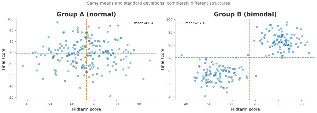
The lesson isn’t subtle: summary statistics alone hide the shape of your data. A mean and a standard deviation can’t distinguish a normal distribution from a bimodal one, a dinosaur, or a circle.
Key Concept: Datasaurus Dozen
Matejka, J. & Fitzmaurice, G. (2017). Same stats, different graphs. Proceedings of CHI 2017. The original Anscombe’s Quartet dates from 1973. Both show the same principle: visualize before summarizing. A modern corollary for ML: never report only RMSE without looking at a residual plot.
# Demonstrate "same stats, different shapes" with two student subsets# that have matching means and standard deviations but different distributions.rng = np.random.default_rng(7)# Group A: normally distributed scores (typical class)n =200group_a = pd.DataFrame( {"group": "Group A (normal)","midterm": rng.normal(68, 12, n).clip(20, 100),"final": rng.normal(70, 12, n).clip(20, 100), })# Group B: bimodal: two subpopulations merged (e.g. two campuses with different resources)group_b = pd.DataFrame( {"group": "Group B (bimodal)","midterm": np.concatenate([rng.normal(55, 6, n //2), rng.normal(82, 6, n //2)]),"final": np.concatenate([rng.normal(57, 6, n //2), rng.normal(84, 6, n //2)]), })combined = pd.concat([group_a, group_b], ignore_index=True)# Summary stats: almost identicalprint("Summary statistics:")print(combined.groupby("group")[["midterm", "final"]].describe().round(1).to_string())print()fig, axes = plt.subplots(1, 2, figsize=(11, 4), sharey=False)for ax, (name, grp) inzip(axes, combined.groupby("group"), strict=False): ax.scatter(grp["midterm"], grp["final"], alpha=0.4, s=18, color="#0369A1") ax.set_xlabel("Midterm score") ax.set_ylabel("Final score") ax.set_title(name, fontweight="bold") ax.spines[["top", "right"]].set_visible(False)# Annotate means ax.axvline(grp["midterm"].mean(), color="#D97706", lw=1.2, ls="--", label=f"mean={grp['midterm'].mean():.1f}") ax.axhline(grp["final"].mean(), color="#D97706", lw=1.2, ls="--") ax.legend(fontsize=8)fig.suptitle("Same means and standard deviations: completely different structures", fontsize=10, color="#6B7280")fig.tight_layout()plt.show()
Summary statistics:
                  midterm                                            final
                    count  mean   std   min   25%   50%   75%   max  count  mean   std   min   25%   50%   75%   max
group
Group A (normal)    200.0  66.4  10.5  37.8  60.2  66.4  73.9  94.9  200.0  69.0  11.7  31.0  60.7  69.3  76.3  97.1
Group B (bimodal)   200.0  67.4  14.8  38.1  53.2  68.2  81.4  93.2  200.0  70.4  14.5  40.4  56.8  71.0  83.0  97.7
Common Mistake: Reporting only mean ± std for a bimodal distribution
Group B above has the same mean and standard deviation as Group A. A table of statistics alone would show no difference. The scatter plot reveals that Group B is actually two separate subpopulations: a finding with direct intervention implications.
Rule: for any continuous variable you care about, always plot a distribution (histogram, KDE, strip plot, or box plot) before reporting a single number.
Activity 8 - Unmask the Hidden Structure
From university_analytics.csv, compare the distribution of final_score for two programs side-by-side using overlapping KDE plots (or box plots). Before plotting, print the mean and standard deviation for each program. Then reflect: would the statistics alone have revealed the difference?
import seaborn as sns
# ... print stats, then plot KDE for each program ...
# TODO: compare final_score distributions for two programs: print stats, then KDE plot...
Capstone: Rescue a Misleading Chart
Below is a chart with three problems from this notebook stacked together: a truncated y-axis, no axis labels, and matplotlib’s unbranded defaults. Fix all three, then add one caption sentence stating the chart’s single message.
# The chart to rescue. Run this first to see what is wrong with it.fig, ax = plt.subplots(figsize=(5, 3))ax.bar(course_means.index, course_means.values, color=["#4477AA", "#EE6677", "#228833"])ax.set_ylim(50, 66)fig.tight_layout()
Capstone Exercise - Fix the Chart
Fix the y-axis to start at 0
Add an x and y axis label
Apply the house style with configure_matplotlib_style()
Add one print statement with a one-sentence caption stating the chart’s single message
Hint:configure_matplotlib_style() only affects charts drawn after it runs, so call it before plt.subplots(), not after.
# TODO: rescue the chart...print("Caption: ...")
Caption: ...
Further reading
Resource
Why it matters
Tufte, E.R. (1983). The Visual Display of Quantitative Information. Graphics Press.
The original data-ink ratio argument that Section 1 is built on, illustrated with 250 examples
Knaflic, C.N. (2015). Storytelling with Data. Wiley.
The most practical data visualisation book for analysts; the annotated chart examples in Chapter 5 are worth the price alone
Cairo, A. (2012). The Functional Art. New Riders.
A data-journalism perspective on the same tension Section 1 covers: a chart must be accurate and engaging, not one traded for the other
Wilke, C.O. (2019). Fundamentals of Data Visualization. O’Reilly.
Free at clauswilke.com/dataviz: Chapter 17 on “proportional ink” and Chapter 18 on chart junk directly support Sections 1–2 of this notebook
Ware, C. (2012). Information Visualization: Perception for Design, 3rd ed. Morgan Kaufmann.
The perceptual science behind Section 6’s preattentive attributes, already cited inline there
Schwabish, J. (2021). Better Data Visualizations. Columbia University Press.
Covers annotation, layout, and the “sorta spaghetti” problem; strong on the gap between what analysts produce and what executives read
Cleveland, W.S. & McGill, R. (1984). Graphical perception. Journal of the American Statistical Association 79(387), 531–554.
The empirical study that established the encoding hierarchy used in Section 1