A Python loop can normalise 2,400 exam scores. It can. It takes thirty lines, runs ten times slower than it should, and looks nothing like the code the person reviewing your pull request expects to see.
NumPy does it in one: (student_data - student_data.mean(axis=0)) / student_data.std(axis=0). No loop. No temporary variables. The operation, stated directly.
That shape, a short expression operating on an entire matrix, is the syntax that Pandas, scikit-learn, and PyTorch all speak. The standard library tools from Chapter 5 handle exact arithmetic on small collections; this chapter introduces the data structure that handles numbers at scale. Chapter 7 (07-numpy-advanced.ipynb) extends it with broadcasting, vectorisation, and linear algebra.
NumPy (numpy.org) was created in 2005 by Travis Oliphant to give Python scientists the numeric performance of Fortran and C without leaving the language. The idea was simple: store numbers in a contiguous block of memory with a fixed type, and let a thin Python wrapper call heavily optimised C and Fortran routines on that block. Two decades later, nearly every numerical computing library in Python (pandas, scikit-learn, PyTorch, TensorFlow) uses NumPy arrays as its currency.
How it compares
Approach
Speed on large arrays
Readable math
When to use
Python list + loop
Slow (Python objects, GIL)
Verbose
Small collections, mixed types
NumPy ndarray
Fast (C/Fortran, contiguous)
Concise (a * 2)
Numeric data of any size
PyTorch Tensor
Fast (optionally GPU)
Similar to NumPy
Deep learning, autodiff
JAX Array
Very fast (XLA, JIT, GPU/TPU)
NumPy-compatible
Research, differentiable programs
CuPy ndarray
GPU only
NumPy-compatible
Large-scale GPU computing
For everything up to classical ML on a laptop, NumPy is the right level of abstraction. PyTorch and JAX add complexity (device management, gradient tracking) that you don’t need yet.
Already in your environment
NumPy is included in pyproject.toml. If you ever start a standalone project:
Explain why NumPy arrays outperform Python lists for numeric data
Sec. 1
2
Create arrays with array, arange, zeros, ones, and a Generator
Sec. 2
3
Inspect and reshape arrays using shape, dtype, reshape, and stacking
Sec. 3
4
Select data with integer indexing, slicing, and fancy indexing
Sec. 4
5
Filter arrays with boolean masks and np.where
Sec. 5
6
Compute per-column and per-row statistics with axis
Sec. 6
1. Why NumPy? The ndarray
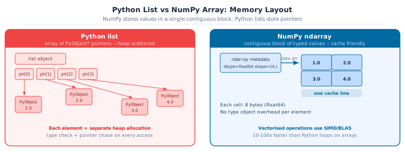
A Python list can hold anything (mixed types, nested objects), which makes it flexible but slow for numeric work: every element is a separate Python object, and arithmetic on a list means a Python-level loop.
A NumPy ndarray (“n-dimensional array”) is different: it stores one fixed dtype in a single contiguous block of memory. That uniformity lets NumPy hand the math off to compiled C/Fortran loops instead of the Python interpreter, often 10-100x faster, and with far less memory per element.
import numpy as npstudy_hours = [12, 5, 18, 9, 22]# A Python list has no element-wise arithmetic: this is string repetition, not math!print("list * 2 :", study_hours *2)hours = np.array(study_hours)print("array * 2 :", hours *2) # element-wise multiplication
Memory layout comparison: Python list stores pointers to scattered heap objects, while NumPy ndarray stores uniform float64 values in a single contiguous block.
A NumPy array is homogeneous (one dtype for every element) and has a fixed shape. Because elements sit next to each other in memory, NumPy can vectorise operations: apply one compiled loop to the whole array instead of looping in Python.
Lists are general-purpose containers; arrays are numeric data structures. Use a list for a heterogeneous bag of objects, an array for a column of numbers.
Activity 1: ndarray vs list arithmetic
Feel the difference between Python lists and NumPy arrays.
Steps: 1. Create scores_list = [78, 85, 92, 91, 55] and scores_arr = np.array(scores_list). 2. Compute the z-score: (scores_arr - scores_arr.mean()) / scores_arr.std(). 3. Confirm the result has mean ~0 and std ~1 using .mean() and .std(). 4. Try scores_list - scores_list[0] and note the error.
Expected: z-scores around [-0.3, 0.3, 1.1, 0.9, -2.0].
2. Creating Arrays
The most direct way to create an array is np.array() from a Python list (or list of lists, for 2D data). For larger or synthetic data, NumPy provides dedicated creation functions so you never have to type out values by hand.
Key Concept: use default_rng, not the legacy random API
rng = np.random.default_rng(42) creates an independent, reproducible stream. The legacy np.random.seed(42) sets global state shared by every library in your process: a hidden coupling that makes results hard to reproduce. Prefer default_rng for all new code.
Synthetic data and simulations need reproducible randomness. Modern NumPy (1.17+) recommends np.random.default_rng(seed) over the legacy np.random.seed(...). A Generator object is self-contained, so two generators never interfere with each other’s state (unlike the old global np.random.seed, which silently affects every call anywhere in the program).
np.random.seed(42) mutates a single global random state shared by your whole program. Any other code (or library) calling np.random.* shifts that shared state and breaks your reproducibility. rng = np.random.default_rng(42) gives you an isolated generator: pass it around explicitly, and your results stay reproducible no matter what else runs.
Activity 2: build a synthetic student dataset
Using rng = np.random.default_rng(7), generate a student_data array of shape (50, 3) for 50 students with columns:
study_hours: rng.uniform(0, 25, size=50)
attendance_pct: rng.uniform(50, 100, size=50)
prior_gpa: rng.uniform(2.0, 4.0, size=50)
Combine the three 1D arrays into one (50, 3) array with np.column_stack.
Hint:np.column_stack([a, b, c]) stacks 1D arrays as columns of a 2D array.
rng = np.random.default_rng(7)study_hours = rng.uniform(0, 25, size=50)attendance_pct = rng.uniform(50, 100, size=50)prior_gpa = rng.uniform(2.0, 4.0, size=50)student_data = ... # TODO: combine the three arrays into one (50, 3) array# print(f"student_data.shape : {student_data.shape}")# print(f"student_data[0] : {student_data[0]}")
3. Shape, Size, and dtype
Every array carries metadata you should check before trusting a computation: shape (size along each dimension), ndim (number of dimensions), size (total element count), and dtype (the single data type of every element).
Key Concept: check .shape and .dtype before any computation
Shape mismatches and dtype surprises are the most common silent NumPy bugs. A (5, 3) array minus a (3, 5) array either errors or broadcasts in a way you did not intend. Print arr.shape, arr.dtype whenever a result looks wrong.
Common Mistake: mixed int/float input silently upcasts
np.array([1, 2, 3.5]) produces a float64 array, not a mix of int and float. NumPy must pick one dtype for the whole array and silently widens every element to fit. This is usually harmless, but np.array([1, 2, 3], dtype=np.int32) / 2 truncating, or an unexpected int8 overflowing past 127, are the same root cause: always check .dtype when results look wrong.
Reshaping
reshape() returns the same data viewed with a different shape. It doesn’t copy or reorder values, so the total element count (size) must stay the same. -1 tells NumPy “infer this dimension from the others”:
x = np.arange(12)print(f"x : {x} shape={x.shape}")x_grid = x.reshape(3, 4)print(f"reshape(3,4):\n{x_grid}")# -1 means "figure this dimension out for me"x_col = x.reshape(-1, 1) # turn a 1D array into a single columnprint(f"reshape(-1,1) shape: {x_col.shape}")x_flat = x_grid.flatten() # back to 1D - always returns a COPYprint(f"flatten() : {x_flat}")
Common Mistake: reshape() returns a view, flatten() returns a copy
Mutating the result of .reshape() mutates the original array too. They share the same underlying memory. .flatten() always copies, so mutating it is safe. This distinction (view vs. copy) comes up constantly in NumPy; Sec. 11 covers it in more depth.
original = np.arange(6)view = original.reshape(2, 3)view[0, 0] =99# mutating the reshaped VIEW...print(f"view :\n{view}")print(f"original : {original}") # ...also changed the original!
Assembling separate 1D arrays into one 2D matrix, or stacking two matrices together, is a common pattern. Use the right function for the shape change you want:
Function
Effect
np.column_stack([a, b, ...])
1D arrays -> columns of a 2D array
np.hstack([a, b])
Join side-by-side (same number of rows)
np.vstack([a, b])
Stack on top of each other (same number of columns)
np.concatenate([a, b], axis=...)
General join along a chosen axis
gpa = np.array([3.1, 2.4, 3.8, 2.9])attendance = np.array([85, 60, 95, 70])# Two 1D arrays -> one (4, 2) matrixcombined = np.column_stack([gpa, attendance])print(f"column_stack:\n{combined}")# Two (4, 2) batches of students -> one (8, 2) matrixmore_students = np.array([[3.5, 90], [2.0, 55]])all_students = np.vstack([combined, more_students])print(f"vstack shape: {all_students.shape}")
Steps: 1. Stack them into a (5, 3) matrix with np.column_stack. 2. Print .shape and .dtype. 3. Reshape to (3, 5) and confirm shapes swapped.
Expected: original shape (5, 3), reshaped (3, 5).
4. Indexing and Slicing
NumPy indexing extends Python’s list slicing to multiple dimensions. For a 2D array, the convention is array[rows, columns], and negative indices still count from the end.
Key Concept: basic slices return views, not copies
Writing sub = student_data[:2] does not copy data: sub shares memory with student_data. Modifying sub[0, 0] = 99 also changes student_data[0, 0]. Call .copy() when you need an independent array.
scores = np.array([62, 78, 85, 91, 55, 73, 88, 95, 67, 80])print(f"first three : {scores[:3]}")print(f"last three : {scores[-3:]}")print(f"between 3 & 7 : {scores[3:7]}")print(f"every other : {scores[::2]}")print(f"reversed : {scores[::-1]}")
first three   : [62 78 85]
last three    : [95 67 80]
between 3 & 7 : [91 55 73 88]
every other   : [62 85 55 88 67]
reversed      : [80 67 95 88 73 55 91 85 78 62]
Common Mistake: basic slices are views; fancy/boolean indexing copies
student_data[:, 1] (a slice) returns a view: mutating it mutates student_data. student_data[1:4, [0, 2]] (a list of indices, known as “fancy indexing”) always returns a copy. If you need an independent array from a slice, call .copy() explicitly: col = student_data[:, 1].copy().
Activity 4: select top performers
Given the student_data array above (columns: study_hours, attendance_pct, prior_gpa), use slicing to print:
The prior_gpa column (all rows)
The first two rows, all columns
The study_hours and prior_gpa columns (skip attendance) for every row
Hint: For (3), use fancy column indexing: student_data[:, [0, 2]].
Comparing an array to a value produces a boolean array of the same shape: a “mask.” Using that mask to index the original array keeps only the True positions. This replaces if/for filtering loops entirely.
Key Concept: use & and | for array logic, not and / or
scores >= 70 and attendance >= 80 raises ValueError on arrays. Write (scores >= 70) & (attendance >= 80). The parentheses matter because & binds tighter than >=.
Combine conditions with & (and) / | (or), not Python’s and/or, which only work on single booleans, not arrays. Each side needs its own parentheses because &/| bind tighter than comparison operators:
at_risk mask : [False False False False False False False False  True False]
n at risk    : 1
np.where(condition, if_true, if_false) builds a new array by choosing between two values element-wise: the vectorised equivalent of a ternary expression inside a loop:
labels = np.where(scores >=70, "pass", "fail")print(labels)# np.select handles more than two outcomesgrade = np.select( [scores >=90, scores >=80, scores >=70, scores >=60], ["A", "B", "C", "D"], default="F",)print(grade)
Given scores and attendance arrays, build a boolean mask needs_help that flags students with score < 70orattendance < 60, then print how many students were flagged and their scores.
mean(), sum(), std(), min(), max() collapse an array to a single number by default. On a 2D matrix, the axis argument controls which dimension gets collapsed: this is the single most common source of “right function, wrong number” bugs in NumPy code, so get the convention straight now:
student_data.mean(axis=0) gives one value per column: per-column statistics. student_data.mean(axis=1) gives one value per row: per-row statistics. Omitting axis collapses everything to a single scalar.
student_data = np.array( [ [12.0, 85.0, 3.1], [5.0, 60.0, 2.4], [18.0, 95.0, 3.8], [9.0, 70.0, 2.9], [22.0, 98.0, 3.9], ])print(f"overall mean : {student_data.mean():.2f}") # one number, all 15 valuesprint(f"per-column mean : {student_data.mean(axis=0)}") # shape (3,): one per columnprint(f"per-student mean : {student_data.mean(axis=1)}") # shape (5,): one per rowprint(f"per-column std : {student_data.std(axis=0)}")print(f"per-column min/max : {student_data.min(axis=0)} / {student_data.max(axis=0)}")
“axis=0” is easy to misremember. Read it as: “collapse axis 0 (the row axis): what’s left is one value per column.” If you want one statistic per column (the usual case before normalising a student data matrix), that is always axis=0.
Activity 6: per-column and per-row statistics
Compute aggregations along both axes.
Using the student_data array from Activity 3: 1. Compute the mean and std of each column (axis=0). 2. Compute each student’s mean score across all columns (axis=1). 3. Z-score normalise the entire matrix with one expression: student_data_z = (student_data - student_data.mean(axis=0)) / student_data.std(axis=0) 4. Confirm student_data_z.mean(axis=0) is all zeros (within floating-point tolerance).
What’s Next
Chapter 6 covered the NumPy fundamentals: creating arrays, shapes, indexing, masking, and aggregations. Chapter 7 (07-numpy-advanced.ipynb) builds on these with the four topics that make NumPy genuinely powerful: broadcasting, vectorisation, linear algebra, and common gotchas.
7. Capstone exercises
Apply everything from this notebook together. Each exercise is self-contained.
Activity 7: build, normalise, and predict
Using the students dataset below:
Build a (6, 3) array student_data with np.column_stack
Z-score normalise student_data (Sec. 6)
Predict exam_score with the given weights/bias using @ (Sec. 9), applied to the normalised data
Compute the RMSE against actual_scores using np.linalg.norm