load_data: (342, 365, 48) (customers, days, half-hours)| Chapter 4's 5 Archetypes, Reused Directly | |
| Archetype | Customers |
|---|---|
| 0 | 64 |
| 1 | 104 |
| 2 | 74 |
| 3 | 50 |
| 4 | 50 |
| n = 342 real AusNet customers, KMeans(k=5) on peak-normalized 90-day shape | |
This chapter asks two real questions: does integrating customer archetype information actually improve load forecasting accuracy for a customer the system already knows, compared to a global or per-customer baseline? And what is the most effective way to forecast electricity demand for a brand-new customer with no historical data at all?
Chapter 1 established an uncomfortable baseline: for 70% of AusNet’s 342 real customers, the simplest possible baseline, a plain window average with no training at all, already wins. A trained model earns its cost only if it clears that floor, and clearing it is only half of what a Distribution System Operator (DSO) actually needs from a deployment. The other half never shows up in an accuracy table: a new house connects tomorrow with zero history in any trained model, and something has to forecast it on day one anyway. This chapter checks both questions honestly on the same real customer pool, rather than assuming a trained model wins or that a clustering idea that looks good on paper survives contact with a customer it has never seen.
Same real AusNet pool Chapter 1 used, no new fetch step. This chapter also reuses Chapter 4’s own customer archetypes directly: KMeans(n_clusters=5, random_state=0) on each customer’s peak-normalized 90-day seasonal shape, the same recipe and the same k Chapter 4 settled on after comparing cluster-validity scores across candidate values, not the Improved Deep Embedded Clustering (IDEC) autoencoder variant Chapter 4 only used for a k-selection comparison.
A little notation, defined once, used throughout: customer \(i\)’s own peak-normalized shape is \(s_i \in \mathbb{R}^{48}\) (Chapter 4’s own recipe, the mean 30-minute profile across a real 90-day season, divided by its own peak), and \(c_1, \dots, c_5\) are the five archetype centroids KMeans fit on the full real population of these shapes. Customer \(i\)’s distance to archetype \(k\) is simply \(d_{i,k} = \lVert s_i - c_k \rVert_2\), a real, checkable number for every customer, known or new. Every mechanism below is really just a different answer to one question: what should a model do with \(d_{i,k}\)?
Key Concept
Clustering and forecasting combine differently depending on whether a customer is known or new. For a customer the system already has real history for, \(d_{i,k}\) is a static feature that legitimately doubles as a personalization signal inside a single shared model, since the model has already trained on that exact customer’s own values. For a brand-new customer, that same feature is meaningless on its own, there is no signature yet to personalize against, and the right mechanism is a distance-weighted blend of already-trained specialists, gated by a calibrated check for whether a real match even exists. That check is a split-conformal threshold, not a grid search: calibrated once on a held-back slice of known customers so that it covers 90% of their own real nearest-neighbor distances, the same finite-sample, distribution-free guarantee [1] Chapter 5 already built for its own retrieval work, reused here rather than re-derived.
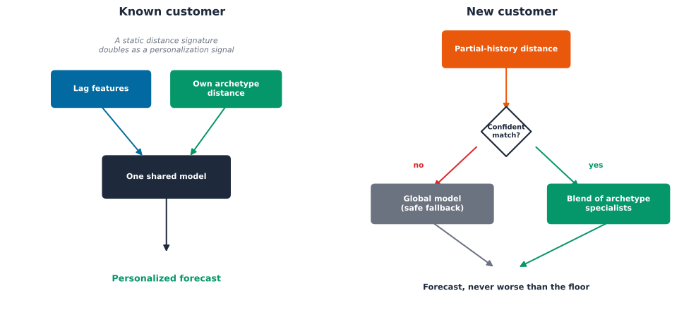
Three approaches, compared honestly on the same 342 real customers and the same last-90-day holdout Chapter 1 used, differing only in how, or whether, \(d_{i,k}\) enters the model:
twiga.models.ml LightGBM model [2], one shared \(\theta\) fit across everyone pooled together, no archetype information at all.\(x_{i,t}\) is the same lag-and-calendar feature recipe Chapter 1 built for feature-importance ranking, put to its first real use training a model, across all three.
Unified wins on MAE, RMSE, Corr, and WMAPE, and is effectively tied on SMAPE, real but modest margins, not dramatic ones: about 0.6% lower MAE and WMAPE than the blind floor, 1.6% lower RMSE, and a real correlation gain of roughly 3%, similarly modest against hard-routing to five separate archetype-specific models. Small margins, but they hold in the same direction on every metric, and they come without needing five separate models to maintain in production, a real operational value: one artifact to version, monitor, and retrain, not five. This matches a broader finding in the forecasting literature: a single model that shares statistical strength across many related series, rather than a strictly local model per series, has repeatedly shown surprising accuracy on grouped time series [3]. But this comparison has every customer’s own real history inside the training pool. That is a fair test of whether profiling helps for a customer already known to the system, not of a customer it has never seen before, and those are genuinely different questions.
“Wins on four metrics, ties on the fifth” is still five separate numbers a reader has to weigh by eye. Chapter 1 of this part turned that same weighing act into a formal, repeatable method rather than a prose judgment call: rank every candidate on every metric, then combine the per-metric ranks into one score, weighted by how much each metric disagrees with the others, \[ u_j = 1 - \frac{1}{J-1}\sum_{j' \neq j} \left|\rho_S(M_j, M_{j'})\right| \] \[ w_j = \frac{u_j}{\sum_{j'=1}^{J} u_{j'}} \] \[ \text{score}(m) = \sum_{j=1}^{J} w_j \cdot \text{rank}_j(m) \] so that MAE, RMSE, WMAPE, and SMAPE, which largely agree with each other here, do not collectively outvote Corr, the one metric asking whether a model tracks the real signal’s shape rather than just its average level.
Unified comes out on top of this diversity-weighted ranking too, the same verdict the five-metric table already gave by eye, now backed by an explicit score rather than a reader’s own five-way judgment call. That agreement is itself worth noting: unlike Chapter 1’s own baseline comparison, where the formal ranking overturned the MAE-only answer, here the two methods agree because unified’s own win is not built on a single metric’s fluke, it holds in the same direction across all five, exactly the situation in which no amount of metric-weighting machinery should be expected to change the answer.
A single train/test split is a snapshot, not a guarantee. The real check for whether unified’s win above is a genuine pattern, and not an artifact of exactly where a 90-day holdout happens to start, is expanding-window backtesting: train on a growing window of real history, test on the next real month, repeat, the same rolling-origin evaluation protocol Twiga’s own backtesting tutorial recommends. Three folds here, each ending before the headline holdout above ever begins, so this check and that comparison never share a single test row.
Unified beats the blind floor in all three expanding-window folds, not only in the final 90-day holdout used above. That is real evidence this is a genuine pattern rather than an artifact of one arbitrary split, checked the same way Twiga’s own backtesting tutorial recommends checking any forecasting claim before trusting it. The same diversity-weighted ranking used throughout this chapter applies here too, averaged across the three folds:
Unified wins the formal ranking as well, the backtest is not just an MAE story repeated three times.
A DSO onboarding a new house tomorrow has no history for it in any trained model. The obvious idea is to reuse the unified model exactly as it is: compute the new house’s own \(d_i\) from whatever real history exists, and feed those distances into the same model. Checked directly, before trusting it.
The diversity-weighted ranking agrees with the raw MAE table: this is not a case where a different metric would have told a kinder story, global blind wins outright, on error and on tracking the real signal alike.
Even at 90 real days of history, exactly matching the full season used to build the archetype centroids in the first place, the unified model is still worse than the global blind model that ignores archetype information entirely. More history does not fix it. The distance features are not being ignored either, a direct feature-importance check shows LightGBM splits on them about as often as it splits on the lag features. What is actually happening is a real, checkable form of overfitting: for a known customer, \(d_i\) is close to a fixed, near-unique vector across every one of their own training rows, so the tree learns to recognize which known customer a row came from rather than what archetype behavior generalizes. That is a legitimate personalization signal for a customer the model has already trained on, exactly the win above, and exactly the wrong signal for a customer it has never seen: there is no signature to recognize yet.
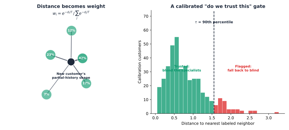
The fix keeps every trained archetype specialist \(f_k\) from the comparison above but stops asking a single model to reason about static per-customer distances at all. Instead, it blends the five specialists’ own predictions directly: \[\hat{y}_{i,t+h} = \sum_{k=1}^{5} w_{i,k} \, f_k(x_{i,t}; \theta_k), \qquad w_{i,k} = \frac{e^{-d_{i,k} / T}}{\sum_{j=1}^{5} e^{-d_{i,j} / T}}\] a softmax over negative distance, sharper toward a single archetype as the temperature \(T\) shrinks, the same mixture-of-experts principle Jacobs, Jordan, Nowlan and Hinton introduced for gating specialist networks by how well each one fits a given input [4], here gated by real archetype geometry instead of a learned gating network. Before trusting this blend at all, it passes through a calibrated gate reused verbatim from Chapter 5, not reimplemented: a split-conformal threshold \[\tau = \text{Quantile}_{1-\alpha}\Big(\big\{\, \min_k \lVert s_j - c_k \rVert : j \in \text{calibration set} \,\big\}\Big)\] computed once on a held-back slice of known customers. Under the same exchangeability assumption behind every split-conformal guarantee in this book [1], at least \(1-\alpha\) of an exchangeable population’s own true nearest-centroid distances fall at or below \(\tau\) by construction, so a new customer whose own distance clears \(\tau\) is trusted with that same finite-sample confidence; one who does not safely falls back to the blind model instead of a confident-looking guess.
Key Concept
Two mechanics carry the whole fix. Distance becomes weight through the softmax above, letting a genuinely ambiguous customer draw on several archetypes at once rather than being forced into one. And the calibrated threshold \(\tau\) decides, honestly and quantitatively, whether there is enough real information to trust that blend at all, rather than assuming there always is.
Population averages are easy to state and hard to feel. One customer from the 72 held out above shows what the gate actually tracks: not whether the single nearest archetype label happens to be correct, but whether a real, trustworthy match exists at all. The gate starts trusting this customer at 7 real days, well before their own hard archetype label finally turns correct at a full season, and the forecast improves exactly when trust arrives, not when the label does.
Zooming out from one customer to all 72 held out entirely from training:
Four candidates this time, not two, the richest comparison in this chapter, so the diversity-weighted ranking earns its keep here more than anywhere else so far:
Gated soft mixture comes out on top, averaged across all five history lengths, the same verdict the MAE chart already suggested, now checked against Corr and RMSE too rather than taken on faith from one column.
Two more real numbers explain the shape of that chart.
The gated soft mixture is never worse than the blind floor at any history length, including a single real day, where the calibrated gate correctly trusts nothing yet and defers entirely. As real history accumulates, both the archetype-assignment accuracy and the retrieval-confidence trust rate climb together: 32% and 0% at one day, 100% and 92% at a full season, and the gated mixture’s own accuracy improves in step, ending as the best of the four approaches by a full season. The practical value is a deployment guarantee, not just an accuracy number: a DSO can forecast a new house from day one with no risk of doing worse than the safe default, and the forecast keeps improving on its own as real meter readings accumulate, with no manual intervention or retraining decision required.
Two different answers to how clustering and forecasting should combine, and which one is right depends entirely on whether a customer is known or new, checked rather than assumed either way. For a customer the system already has any real history for, a single model that receives \(d_i\) as ordinary features wins outright, because that static distance signature legitimately doubles as a personalization signal. For a customer with no history in any trained model yet, that same mechanism actively fails, even with a perfect archetype match, because there is no signature yet to personalize against. The fix reuses machinery this book already built rather than inventing new machinery: Chapter 4’s archetype centroids supply \(d_i\), Chapter 5’s own calibrated retrieval-confidence check supplies the honest “do we actually have a close real match” gate, and the two combine into a soft, distance-weighted blend of the same specialist models trained above. It is never worse than doing nothing, and it gets measurably better as real history accumulates, exactly the property a genuine day-one deployment needs.
A DSO does not get to choose between accurate and operationally maintainable, and does not get to wait for a new customer to accumulate a full season of history before forecasting them at all. The real, checked finding here is that both constraints have one honest answer each: reuse a single model with cluster information as a legitimate personalization signal once a customer has real history, and fall back to a calibrated, distance-weighted blend of already-trained specialists, safely gated, before that history exists. Neither answer was assumed going in. The first naive idea this chapter tried, reusing the same personalization mechanism for new customers, failed a genuine held-out test even with perfect information, and the fix that replaced it reuses machinery Chapters 4 and 5 already built rather than adding anything new.
Two honest limits, not yet solved here rather than papered over. The archetypes themselves are a snapshot: if a customer population’s own behavior shifts substantially, the centroids this chapter reuses from Chapter 4 would need recomputing, not assumed to stay valid forever. And a genuinely atypical new customer, one whose real behavior does not resemble any of the five archetypes, is exactly the case the retrieval-confidence gate is built to catch: it falls back to the safe global model rather than forcing a bad match, but a low-trust customer still only gets the blind floor, not a personalized answer. Both are real, open questions for a future chapter, not solved by this one.
A trained model clears Chapter 1’s baseline floor, and sharing information across Chapter 4’s archetypes inside a single model beats both training one model per customer and training one model for everyone. That same sharing mechanism does not survive contact with a customer it has never seen, and the fix that does, a calibrated, distance-weighted blend of specialists, is never worse than doing nothing while a new customer’s history accumulates. Chapter 3 picks up the model this chapter found actually earns its cost and asks what that forecast is worth without a number attached to how wrong it might be; Part 8 Chapter 4 asks a further question neither chapter can answer on its own, whether a foundation model pretrained on none of this data, given no fitting step at all, gets the same customers wrong that this chapter’s trained model does.