Chapter 4: Multi-Task Deep Learning at Low Frequency
A kettle switches on. Not as a crisp current transient at 30kHz, the kind Chapters 2 and 3 built their whole pipeline around, but as a slow rise in a number a real smart meter reports once every few seconds. There is no before-window and after-window to subtract, no single clean event to isolate: a fridge is already cycling, a dishwasher is running, and the kettle’s own contribution is just one more wrinkle in a continuously wandering aggregate curve. This is the low-frequency world Chapter 1 named and Chapter 3 handed off to: energy estimation, not load identification, at the rate every real smart meter actually reports.
The question changes with it. Not “which appliance is this event,” not even “which appliances are active in this window” (Chapter 3): now, how much power is each one drawing, continuously, moment to moment, alongside whether it is on at all.
From one state to a state and a power
An aggregate reading is still the same sum Chapters 3 and 4’s own source papers both start from,
\[ x_t = \sum_{m=1}^{M} y_m(t) \cdot s_m(t) + \epsilon_t, \]
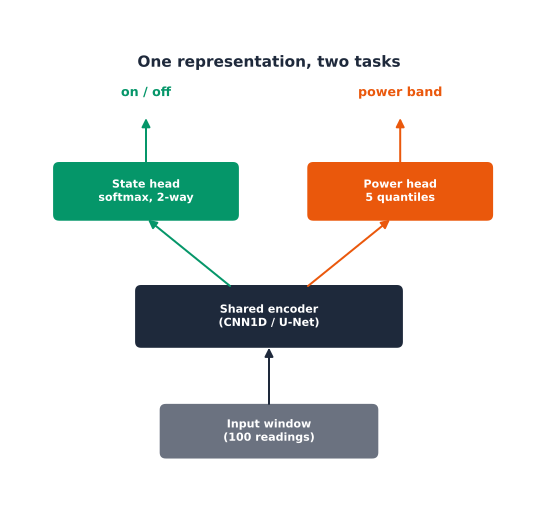
but now each appliance \(m\) carries two targets instead of one: a binary state \(s_m(t) \in \{0, 1\}\) and a continuous power \(y_m(t)\), one derived directly from the other by a fixed threshold. That coupling is the actual argument for a multi-task model: one shared representation feeding two heads, rather than a classifier and a regressor trained as if they had nothing to do with each other [1].
Five real UK-DALE house-1 appliances make this concrete: kettle, fridge, dishwasher, washing machine, microwave, the same subset and the same house the source paper itself uses.
Turning a power curve into a state
Above a fixed on-power threshold (2000W for the kettle, the real constant this data was built from), a continuous curve becomes a binary label. That threshold is not something the model has to discover; it is how the ground truth itself was built.
From an activation window to a sliding window
Chapters 2 and 3 isolated one detected event: a before-window and an after-window around a single state change. There is no event to detect at low frequency, so a fixed window of 100 consecutive aggregate readings slides across the whole signal instead, and the target is the state and power at the window’s last point, a seq2point framing, matching the Dataset class in the author’s own UNETNiLM repository. That repository builds windows one at a time in Python; at this chapter’s scale, hundreds of thousands of candidate windows rather than Chapters 2-3’s few thousand activations, that loop is a real bottleneck, so this notebook gathers every window with one vectorized NumPy operation instead.
Two backbones, one set of heads
Key Concept
Multi-target quantile regression is not five separate regressions bolted together. A single shared network predicts a handful of quantiles per appliance at once (here, the paper’s own choice: 2.5%, 10%, 50%, 90%, 97.5%), trained with the pinball loss, which penalizes over- and under-prediction asymmetrically depending on which quantile is being fit: \[ \mathcal{L}_\tau(y, \hat y) = \begin{cases} \tau \cdot (y - \hat y) & y \ge \hat y \\ (1-\tau) \cdot (\hat y - y) & y < \hat y \end{cases} \] for quantile level \(\tau \in (0, 1)\), real power \(y\), and the model’s own prediction \(\hat y\) for that quantile. A low \(\tau\) (e.g. 0.025) penalizes over-prediction nine times more than under-prediction; a high \(\tau\) (e.g. 0.975) does the reverse; \(\tau=0.5\) recovers plain absolute error. The payoff: a real uncertainty band around every prediction, not just a point estimate, at essentially no extra modeling cost over a plain regression head [1].
Both backbones compared here end in the identical pair of heads: a per-appliance 2-way softmax for state, the same mechanism Chapter 3 used for multi-label appliance state, and a per-appliance multi-quantile linear head for power. The two backbones differ only in how the shared representation \(h\) gets built from the input window \(x\). CNN1DModel is a plain stacked encoder, each layer’s output feeding directly into the next with nothing carried across: \[
h = f_L\big(f_{L-1}(\cdots f_1(x) \cdots)\big).
\] UNETNiLM is a true U-Net: the same downsampling stack \(f_1, \dots,
f_L\), followed by an upsampling stack \(g_L, \dots, g_1\) where each upsampling layer concatenates its input with the matching downsampling stage’s own output before deconvolving, \[
h_l = g_l\big([\, h_{l+1} \, ; \, f_l(x) \,]\big),
\] \([\cdot\,;\,\cdot]\) denoting channel-wise concatenation, so a detail computed early in the downsampling pass is available directly to the matching upsampling layer, not only through everything in between. Ported directly from the author’s own UNETNiLM repository, with two small fixes applied along the way: the checked-out unet.py imports Conv1D/Deconv1D from a .block module that does not exist (they live in layers.py), and its U-Net class referred to an undefined num_classes that needed to be a constructor argument. Both are one-line fixes, not a redesign; everything else is the original architecture, verified directly against the code, not just the paper’s prose.
Live results: does the U-Net actually help here?
Both models trained on a real subsample of the UK-DALE training split (100,000 windows, far short of the full 1.5 million-plus readings available, but enough to train on real data throughout) and evaluated on a held-out 20,000-window test subsample. MAE below is in the same per-appliance normalized units both models were trained on, not raw watts; NDE is a ratio and unaffected either way.
Inconclusive, at this training budget, and that is itself the honest result. In this run, CNN1DModel has the lower (better) MAE on four of five appliances, kettle, fridge, dishwasher, and washing machine, UNETNiLM only winning on microwave, and the lower NDE on all five. State detection is close to a tie: macro F1 65.9% for CNN1DModel against 65.7% for UNETNiLM, example-based F1 33.1% against 30.9%. Re-executing this exact code, same seed, same data, produced four different rankings across four runs while this chapter was being written: macro F1 ranged 64.5-68.7% for CNN1DModel and 65.7-68.9% for UNETNiLM, overlapping ranges with no consistent winner, sometimes UNETNiLM ahead by three points, sometimes CNN1DModel ahead, purely from ordinary CPU floating-point non-determinism in convolution and batch-norm reduction order. The published result finds a clear, repeatable U-Net advantage, average MAE reduced 26.35% and F1-macro 0.941 against 0.930 for the plain CNN baseline, on a training budget far larger than this chapter’s 100,000 random windows across 6 epochs afford [1]. At book scale, that gap is too small relative to run-to-run noise to call reliably in either direction; the architecture question needs either more training or a less noisy evaluation to answer here, not a bigger claim than the data supports.
A close look at uncertainty
One real kettle activation from the held-out test split, predicted by UNETNiLM as a full set of quantiles, not just a single number. The 80% and 95% bands come directly from the same multi-quantile head trained above, nothing extra fit on top.
Checking the combined loss itself
The two task losses are summed unweighted, matching the paper’s own choice: \[ \mathcal{L} = \mathcal{L}_{state} + \mathcal{L}_{power}, \] \[ \mathcal{L}_{state} = \text{CE}(s, \hat s), \qquad \mathcal{L}_{power} = \sum_{\tau} \mathcal{L}_\tau(y, \hat y_\tau), \] the state term a plain cross-entropy between the true and predicted state \(s\), the power term a sum of the pinball loss above across every quantile level \(\tau\) the power head predicts. No weight in front of either term, worth checking directly rather than assuming neither one quietly dominates the other.
Both terms decrease smoothly across every epoch for both backbones, and if anything the state (cross-entropy) loss stays two to three times larger than the power (pinball) loss throughout training, not the other way around. Nothing here suggests one task is starving the other, at least at this scale.
What “reproducible benchmarking” means here
DeepNLMTK.pdf is not where this chapter’s model code came from. Deep-NILMtk’s own UNETNILM* variants turned out to be single-task regression or mixture-density models, no joint state head at all, and its multi-task attention variant has a constructor signature mismatch that would fail on instantiation. What the toolkit paper is used for here is its actual contribution: a standardized template for comparing NILM models fairly, same split, same metrics, same held-out test set, model differences isolated from data or evaluation differences [2]. That discipline is exactly what the CNN1DModel vs UNETNiLM comparison above followed: identical heads, identical data, identical training budget, only the backbone differs.
Why bother
Three concrete things this buys beyond “another architecture.” First, deployability taken one step further than Chapter 3: no event detector at all is needed now, this works directly off the low read-rate every real smart meter already reports, not a high-frequency stream most utilities will never collect. Second, multi-task efficiency: one shared model instead of five separate single-appliance models to train, version, and keep working, a real engineering cost that compounds at fleet scale. Third, actionable uncertainty: a quantile band, not a point estimate, is what a downstream system, a demand-response signal, an anomaly flag, an appliance-health check, needs to decide how much to trust a specific prediction at a specific moment, not just on average across a test set.
Where this part of the book goes
This closes Part 2. The quantile regression this chapter leaned on is not a one-off trick: Part 3’s forecasting chapters, built on Twiga, reuse the same idea for a different target, whole-house load instead of per-appliance power, with the same payoff of a real uncertainty band instead of a single number.
Common Mistake
Reporting one training run’s number as if it settles an architecture comparison, instead of checking whether the gap between architectures is larger than the run-to-run noise. It usually is not, at this scale: two close architectures and a light training budget together mean ordinary CPU floating-point non-determinism in convolution and batch-norm reduction order can move the result more than the architecture choice does. A single confident-looking decimal is not evidence of anything until it survives being re-run.