Chapter 3: Multi-Appliance Recognition
A coffee maker clicks on. Before its heating element has even settled into a steady draw, the kettle across the counter finishes boiling and clicks off, and the fan in the next room is still running from twenty minutes ago. One current window, three appliances, two of them mid-cycle already. Chapter 2’s whole pipeline, the before-window, the after-window, the subtraction that isolates exactly one appliance’s signature, quietly assumed this never happens: that whatever changes in a window is caused by exactly one appliance switching state. Real homes do not clear that assumption. They rarely change one thing at a time.
This chapter keeps the tools Chapter 2 built, activation windows, PAA, distance-similarity matrices, a small CNN, but asks a different question of them. Not “which one appliance is this,” but “which appliances, plural, are active right now.” That is a genuinely different problem, not a harder version of the same one, and it needs a different label, a different metric, and one new piece of signal processing to answer well.
From one label to a set of labels
Chapter 2’s classifier picked exactly one class per activation. That stops making sense the moment more than one appliance can be active in the same window: the aggregate current a classifier sees is the sum of whatever is running, not a clean sample of one appliance. The right target is a state vector, one entry per appliance, each either on or off, not a single class index. Given aggregate measurements \(x_t\) built from \(M\) appliances, each with its own power draw \(y_t^{(m)}\) and state \(s_t^{(m)} \in \{0,1\}\),
\[ x_t = \sum_{m=1}^{M} y_t^{(m)} \cdot s_t^{(m)} + \epsilon_t \]
the job is to recover the whole state vector \(\mathbf{s}_t\), not one label, from one aggregate feature vector [1].
Key Concept
Macro \(F_1\), the metric Chapter 2 used throughout, still works here: it scores each appliance separately and averages, so an appliance that is almost always off does not get to hide behind one that is almost always on. But multi-label prediction has a second, equally real question macro \(F_1\) cannot answer on its own: for this one activation, did the model get the whole set right, not just each appliance’s own average? Example-based \(F_1\) (\(F_1\)-eb) answers that instead, scoring each sample’s predicted set against its true set and averaging over samples. A model can score well on one and poorly on the other: high macro \(F_1\) with a few appliances it never gets right in combination, or high \(F_1\)-eb with one rare appliance it silently ignores. Both numbers matter; neither replaces the other.
Does the same feature carry over as-is?
The obvious first move is to reuse Chapter 2’s own two representations, the binary V-I image and the raw activation current, and just see what happens once “the current” might be more than one appliance’s signature added together. The plot below is a real PLAID event with two appliances already active in the same window.
Training the same small CNN on both representations, on a real, multi-label subset of PLAID (1154 aggregated activations, each labeled with every appliance active in the background, not just whichever one changed state [1]), gives a real answer rather than an assumed one.
V-I image reaches 65.7% macro \(F_1\); raw activation current reaches 62.7%. That is not the order the published result found, current a few points ahead of V-I there too [1], but the published gap between them is itself small (0.826 to 0.849), and this run’s own gap is just as small in the other direction. Read it as what it is: two representations that are genuinely close, not one cleanly beating the other. Neither is good enough to call this problem solved.
Fryze power decomposition
The fix is not a bigger network. It is a real piece of signal processing Chapter 2 never needed: splitting the current itself into two physically different parts before any image gets built. The Fryze power theory decomposes an activation current \(i(t)\) into an active component, purely resistive, in phase with the voltage, and a non-active component, whatever is left over [1]:
\[ i(t) = i_a(t) + i_f(t) \]
The active component carries the same active power as the real signal, at the same voltage:
\[ i_a(t) = \frac{p_a}{v_\text{rms}^2} \, v(t), \qquad p_a = \frac{1}{T_s}\sum_{t=1}^{T_s} i(t) \, v(t) \]
and the non-active component is simply what remains, \(i_f(t) = i(t) - i_a(t)\). Two appliances sharing a window rarely agree on both of these at once, even when their raw sum looks similar. The plot below applies this split to the same two-appliance event shown above.
From decomposed current to a distance matrix
Chapter 2’s distance_matrix() step reappears unchanged. It is applied separately to the active and non-active components, each PAA-reduced to the same fixed size \(w\), and stacked as two channels the same way Chapter 2 stacked three phases for LILACD. Four representations are compared in total: the V-I image and raw current from above, the decomposed current itself fed directly to a small 1D CNN, and the decomposed current’s own distance-similarity matrix fed to a 2D CNN.
Decomposing the current is what actually moves the number: 79.7% macro \(F_1\) for the decomposed current itself, 77.9% for its distance matrix, both roughly 15 points above either representation that skipped the decomposition. The published result finds the same shape (0.931 and 0.940 macro \(F_1\) against 0.826 to 0.849 without decomposition) and calls the two decomposed features “comparable,” which is exactly what this run finds too: decomposed current and decomposed distance land within two points of each other, in either order [1]. The signal processing step is doing the real work here, not the choice of image on top of it.
The multi-label head, and what its softmax trick actually buys
The usual way to bolt multi-label output onto a CNN is a sigmoid per appliance and a threshold, typically 0.5, that turns a probability into a yes-or-no. That threshold is picked after training, not learned as part of it, and building a better one is its own open problem [1]. The classifier trained above does something more specific instead: it produces two logits per appliance, one for off and one for on, and applies a softmax over just those two before a cross-entropy loss, verified directly against the author’s own training code, not just the paper’s prose.
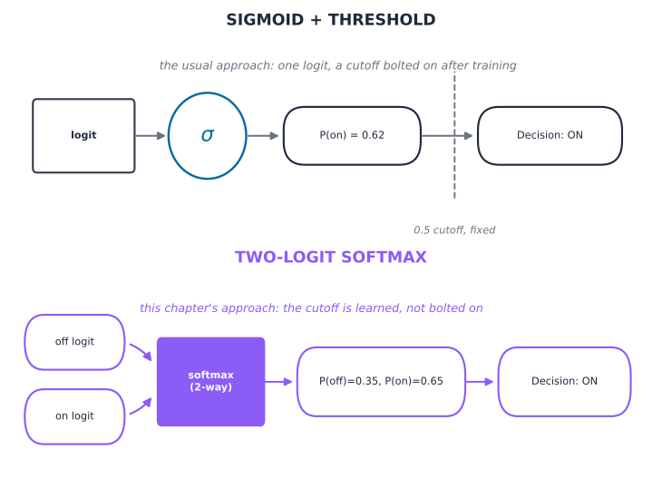
Worth being precise about what that buys, because the honest answer is narrower than it first sounds. Write appliance \(m\)’s two logits as \((a_m, b_m)\), off and on. The softmax probability of “on” is
\[ \hat{p}_m = \frac{\exp(b_m)}{\exp(a_m) + \exp(b_m)} = \frac{1}{1 + \exp(a_m - b_m)} = \mathrm{sigmoid}(b_m - a_m), \]
dividing numerator and denominator by \(\exp(b_m)\). So this is a reparametrized sigmoid, not a fundamentally different mechanism. What is genuinely different is where the decision boundary lives: with two competing logits, “on” wins whenever \(b_m > a_m\), a rule trained end to end as part of the network, rather than an external 0.5 cutoff applied to a probability after the fact. Small difference, but a real one, and it is the one this chapter can defend without overselling it.
One more honest note. The original paper describes this loss as one that “implicitly captures the relations between labels” [1]. Structurally, that is not quite what is happening: each appliance’s two-logit softmax above is computed independently of every other appliance’s, with no term in the loss that couples them directly. Whatever relation the model learns between, say, a kettle and a fan being on together comes entirely from the shared CNN encoder underneath, the same 128 features feeding every appliance’s own logit pair, not from the softmax or the loss itself. Worth knowing before reading more into the mechanism than it delivers.
Which appliances specifically?
Macro \(F_1\) hides which appliances the winning feature still struggles with. Per-appliance \(F_1\), V-I image against the decomposed distance matrix, on the same held-out split.
Most appliances improve substantially: AC, CFL, Fan, ILB, and LaptopCharger all sit under 70% on V-I, some far under it (CFL at 64%, Fan at 52%), and all five clear 70% on the decomposed distance matrix, CFL by nearly 30 points. Appliances already strong on V-I stay strong: HairIron, FridgeDefroster, Fridge, and Vacuum (100% on both). SolderingIron and Waterkettle improve substantially without quite crossing the 70% line, and CoffeeMaker barely moves at all, the one exception the next section explains directly. The published result reports the same broad pattern, over 90% example-based \(F_1\) for every appliance except AC, ILB, and LaptopCharger, once the decomposed distance feature is used [1]. This run’s own weak point is sharper and different in its specifics: CoffeeMaker stays at 19.5% even after decomposition, its worst score by a wide margin. Coffee makers are simple resistive heating elements, the same category of appliance Chapter 2 found genuinely hard to tell apart in LILACD (Raclette and Coffee-machine confused each other more than any other pair there). The same physical reason plausibly applies here, and unlike in Chapter 2, it is checkable directly rather than left as a plausible story.
Why the coffee maker specifically?
Restricting to the 648 single-appliance activations (so each point is one appliance’s own current, not several summed together), the Fryze split gives a direct per-sample measurement: how much of an appliance’s own current is non-active, as a share of its total RMS current. A purely resistive load carries almost no non-active current by definition; a motor or a switching power supply carries much more.
The three lowest scorers on the decomposed distance matrix, SolderingIron, Waterkettle, and CoffeeMaker, are exactly the three appliances with the lowest median non-active share here (8.0%, 8.8%, and 9.0%), clustered on top of each other near zero. AC and ILB, also plain resistive loads, sit close behind at 10.8% and 14.1%. Motors and electronics separate cleanly from all of them: Fridge and HairIron sit in the 30-40% range, and CFL and LaptopCharger, both switching electronics, average above 85%. CoffeeMaker’s weak score is not a modelling failure; it is measuring an appliance whose own current genuinely looks like its resistive neighbours, decomposition or not.
What kind of mistake is it?
A multi-label miss is not one thing. Missing every active appliance is a different failure than mislabeling one of three, and lumping them into a single error rate hides which failure mode actually needs fixing. Following the same taxonomy the original paper used: zero-error (predicts nothing active when something is), one-to-one (gets the single active appliance wrong when only one is running), and many-to-many (confuses at least one appliance when several are active, split further by how many of them it got wrong) [1].
Of 111 incorrect predictions on this held-out split, single-appliance confusions dominate: 68 samples where the model got every active appliance right except one. Zero-errors are rare (16), complete misses rarer still (8), and one-to-one errors, the case where only one appliance is running at all, are the least common failure of any type (9), the same result the published paper found: with over 50% of activations being single-appliance events, the model sees plenty of them and gets almost all of them right. Where this run’s own finding actually diverges from the published one is the many-to-many split itself. The paper reports double-errors as its most common failure; here, single-errors dominate instead. That is plausibly a consequence of the data itself: two-appliance activations outnumber three-appliance ones by roughly four to one, so when the model does slip on a multi-appliance window, the more likely window to slip on is a two-appliance one, where getting one of two wrong is, by construction, a single-error.
Why bother
Two concrete things this buys beyond “now it handles more than one appliance.” First, deployability: single-label recognition has a hidden dependency on a near-perfect event detector, one that guarantees clean, isolated activations. That holds in a curated dataset and fails constantly in a real home, a fridge compressor cycling in the background while a kettle switches on. Multi-label recognition removes that dependency entirely; it does not need the aggregate signal to cooperate.
Second, co-occurrence is itself the information, not just a nuisance to model around. Knowing that a kettle, a hair dryer, and an air conditioner are all drawing power at the same instant is exactly what a time-of-use tariff, a demand-response program, or a circuit-capacity check needs, and it is something a sequence of clean, single-appliance events can never directly answer. Chapter 2’s own “why bother” was one machine’s signature drifting over months, an industrial, predictive-maintenance value. This chapter’s is the residential-facing counterpart: which appliances are drawing power together, right now.
Where this part of the book goes
This chapter and the last both stayed inside the same high-frequency, event-based world: a short activation window, a graph-like or distance-based image, a CNN. Real smart meters mostly do not offer that world at all.
- Chapter 4, deep learning at low frequency, moves off event-based, high-frequency features entirely, onto the energy-estimation side of NILM introduced in Chapter 1, the kind of problem a meter reporting once every few seconds can actually be asked to solve.
Common Mistake
Treating a low per-appliance macro \(F_1\) as one failure with one cause. CoffeeMaker’s 19.5% here and the published paper’s own AC/ILB/LaptopCharger weak points are not evidence that decomposition “doesn’t work”; they are evidence that current-shape features cap out on appliances whose current shape is not very distinctive to begin with, mostly plain resistive loads. Fixing that needs a feature sensitive to something other than current shape, not a longer training run on the same one.