{'converged': True,
'n_buses': 61,
'n_lines': 59,
'n_loads': 31,
'n_transformers': 1,
'total_p_loss_kw': 0.6107992120127365,
'total_q_loss_kvar': 0.15519491021295995}Chapter 2: Time-Series Simulation and DER Modeling
This book’s whole premise is that a smart-meter reading is worth more than its own number: aggregated, modeled, and combined with what a meter alone can’t see, network topology, everyone else’s demand at the same moment, it becomes a real business decision. Chapter 1 built the network side of that combination, an OpenDSS model of a real Low Voltage (LV) feeder, and ended on a warning: one solved snapshot is not a verdict on a feeder’s health.
This chapter is where the meter-signal side of that premise finally meets the network. The same 31-customer AusNet feeder runs across a real week of demand, then answers two business questions: how much rooftop solar, and how much Electric Vehicle (EV) charging, can this specific feeder actually take before someone has to act on it. The two answers turn out to be very different problems, at different times of day, binding on different constraints, and the fix built for the first one does not generalize to the second.
Getting the data
This chapter needs the same AusNet LV network and smart-meter data Chapter 1 introduced, plus one more dataset: EV home-charging profiles. Neither is checked into this repository (someone else’s licensed data, vendored locally instead), so fetch both once before running the notebook:
uv run python scripts/fetch_part4_ausnet_data.py
uv run python scripts/fetch_part4_ev_profiles.py
The first downloads the network model and two datasets, 342 anonymized customers’ active-power readings and their matched normalized Photovoltaic (PV) generation, both at 30-minute resolution for a full year. The second downloads EV home-charging profiles derived from a UK metering trial. That second source ships no license, so this chapter uses it as a reference for building its own scenario, not as data reused verbatim; every number reported below is this notebook’s own.
This chapter’s feeder
Every section below runs on one network: the 31-customer AusNet feeder Chapter 1 introduced, the same distribution transformer, the same 24 line segments and 31 single-phase service cables. A result from the middle of this chapter and a result from the end describe the same physical feeder, not two unrelated ones.
Real customers, real diversity
Before driving this feeder with real data, it is worth seeing what that data actually looks like: not one representative household, but hundreds of different ones.
342 households, one day, and no two profiles agree: some barely draw half a kilowatt all day, others spike past 5kW in the evening. Averaging this away into “the” residential load shape would erase exactly the variability a real feeder has to survive.
PV varies day to day the same way: cloudy days barely clear a third of a clear day’s peak. The hosting-capacity study later in this chapter deliberately picks the single sunniest of these 365 days, the worst case for that particular question.
That diversity is also why this chapter bothers deriving a LoadShape from an actual reading rather than assuming one: a network fed by a made-up “typical” profile would never show the swings the chart above just did.
From readings to LoadShapes
For residential customers, most utilities only bill on active energy, so many residential smart-meter datasets only retain active power, even though the meter hardware could measure more. This dataset reports only active power for exactly that reason; reactive power is derived here from an assumed power factor in the 0.95-0.99 range, the same convention the network’s original tutorial uses.
Every one of the feeder’s 31 loads gets its own customer profile, sampled from the 342 available. Attaching a LoadShape is one command, but trusting it silently is a habit worth breaking: it costs little to cross-check the underlying data array, what a live solve reports back, and what the LoadShape object itself has stored, against each other.
A gap at solver-tolerance scale, well under a watt, confirms all three views describe the same house. Catching a mismatch here is far cheaper than noticing it three sections later in a chart that looks slightly off.
A week of simulation
circuit.solve_daily(steps, stepsize) steps through a Set Mode=daily solve, but a single call only ever covers one day’s worth of LoadShape data. A genuine time-series study covers more than one day, so every LoadShape gets rebuilt at the start of each new day and the solve runs seven times over, a full real week.
Three phases, one real week: demand rises and falls with the daily cycle, and no two days look quite the same, exactly the kind of pattern a single snapshot could never show.
Comfortably inside the 0.94-1.10 pu band all week, no PV yet attached. The rest of this chapter revisits this same feeder twice, once with rooftop solar added, once with EV charging, and the envelope stops staying so comfortable.
Modeling PV properly
A PVSystem can run on a flat rating, constant output regardless of the time of day. A more realistic model drives it from an irradiance profile and a temperature profile instead, attached to an actual house on this same feeder rather than a separate demonstration network.
A 20% default nearly zeroed out the morning and evening. OpenDSS’s PVSystem defaults %cutin/%cutout to 20%, the inverter output threshold below which it will not turn on or stays off. At 10% irradiance, a real inverter still produces something, but a 20%-cutin model reports flat zero, and it is easy to miss unless every hour gets checked individually: the middle of the day looks identical either way. A realistic PV system instead sets %cutin=0.05 %cutout=0.05.
Rebuilding the same PV system with the lower threshold recovers exactly the two hours the default silently dropped.
A single house’s PV system modeled correctly is a technical fix. Whether a whole feeder full of them still passes muster is a business question, and it is the one this chapter has been building toward since the first solved snapshot.
The hosting-capacity crisis
This is the business question a Distribution System Operator (DSO) faces every time a new rooftop solar application arrives: does connecting one more customer’s PV system push this specific feeder past its statutory voltage limit? Say yes too often and customers wait months for a grid upgrade that may not have been necessary; say yes too rarely and a feeder starts violating compliance. A hosting-capacity study is how that question gets a feeder-specific answer instead of a guess.
A feeder can fail this test two different ways, not one. Chapter 1 introduced the three constraints an LV network operates under: thermal, voltage, and phase balance. The notebook’s own run_penetration function checks the first two together at every step, as two real inequalities: \[
\max_i V_{i,pu}(t) \le 1.10, \qquad \max_t \big|S_{transformer}(t)\big| \le S_{rated} = 500 \text{ kVA},
\] the worst bus voltage against the statutory limit, and the transformer’s apparent power against its own 500 kVA nameplate rating.
Day 363 is the sunniest day in the dataset, the tallest curve in this chapter’s own PV diversity chart, and the worst case for a hosting-capacity study: if a penetration level is ever going to cause a violation, a low-demand, high-sun day is where it shows up first.
The feeder-wide maximum stays inside the compliant band through 60% penetration, then crosses the 1.10 pu statutory limit at 80%. That is a real answer to a real question, not a theoretical ceiling: this specific feeder, on its sunniest day, with realistically-sized rooftop systems, can host roughly six in ten customers with solar before it needs an intervention to host more.
Voltage is the constraint that binds first here, but it is worth checking the other one too, since a feeder that passes the voltage test can still fail the thermal one on a different network.
Nowhere close: even at 100% penetration, the transformer peaks under 30% of its 500 kVA rating, an order of magnitude of headroom left. On this feeder, voltage is the real limit, not heat. That is not true of every LV feeder; a longer or more heavily loaded one can hit its thermal ceiling well before its voltage limit, which is exactly why a proper hosting-capacity study checks both rather than assuming one always dominates.
Fixing the crisis
80% penetration is the violation found above. The same scenario, the same 25 PV systems on the same feeder, gets Volt-Watt and Volt-VAr control applied directly rather than a fresh demonstration network. Both are smart-inverter functions standardized by Institute of Electrical and Electronics Engineers (IEEE) 1547-2018 [1], modeled in OpenDSS as an InvControl element driven by an XYCurve of four voltage/output setpoints. A single InvControl with no explicit PVSystemList applies to every PVSystem in the circuit at once, all 25 of them here, no per-house wiring required.
Volt-Watt curtails real-power export once voltage crosses a threshold, a piecewise-linear function of the local bus voltage \(V\): \[ P(V) = P_{rated} \times \begin{cases} 1 & V \le 1.05 \\[4pt] \dfrac{1.10 - V}{1.10 - 1.05} & 1.05 < V < 1.10 \\[4pt] 0 & V \ge 1.10 \end{cases} \] full output stays available up to 1.05 pu, then ramps linearly down to zero at 1.10 pu. It works, but it reduces the total generation exported. Volt-VAr takes a different lever: instead of cutting real power, it asks the inverter to absorb or supply reactive power, the same principle behind Conservative Voltage Reduction, flattening a feeder’s voltage profile without reducing real generation.
Both bring the feeder back under the 1.10 pu line, and Volt-VAr does it without curtailing a single kilowatt of generation. Volt-Watt curtails real power directly; Volt-VAr does not, which makes it the better first option to try before accepting reduced generation.
That single point, 80% penetration, is where the violation happens to show up first, but the question worth asking is bigger than one point: does either control raise the feeder’s hosting capacity across the board, not just patch this one level?
Neither control ever crosses the 1.10 pu line across the entire sweep, all the way to 100% penetration. The 80%-penetration ceiling this section opened with was not a hard limit on the feeder; it was a limit on running PV without mitigation. With either control active, this same feeder can host every customer on it.
Storage: a third lever
Volt-Watt and Volt-VAr both react to a violation the instant it happens. A battery can act ahead of it instead: charge on a sunny midday when PV export is pushing voltage up, discharge into the evening peak when demand is pulling it down. A Storage element is a dispatchable battery, bounded by its own rated power and energy capacity, its output sign set by its commanded state rather than by the weather or the time of day.
The comment in that cell is worth reading as carefully as the code: OpenDSSDirect.py is a singleton engine, one compiled circuit per process, so two Circuit objects can exist in Python at once, but only one of them is ever telling the truth about what is currently solved. Reading each result immediately after its own solve avoided a real version of this bug, caught while drafting this notebook, not just a hypothetical one.
EV demand: the opposite failure mode
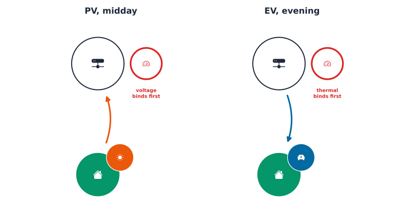
Every section so far has been about PV pushing power out onto the feeder at midday. Electric vehicles push demand the other way: an EV charger is a load, not a generator, and it draws power precisely when a feeder is already under the most strain, the evening, after commuters get home and plug in, right on top of ordinary dinner-time demand. This chapter’s own transformer-loading chart already showed the week’s sharpest peaks land in the evening, before a single EV was in the picture. The question this section asks: does the same feeder that nearly failed a PV test at midday also fail an EV test in the evening, and if Volt-Watt and Volt-VAr fixed the first problem, do they do anything for the second?
This chapter also draws on EV home-charging profiles derived from a UK metering trial: metered charging behavior, not a synthetic assumption, for Level 1 (3.68kW) and Level 2 (7.36kW) chargers, diversified across a group of vehicles to account for the fact that not everyone charges at the same time. The source repository for this data ships no license, unlike the network and smart-meter data behind the rest of this chapter, so it is used here as a reference for building this chapter’s own scenario, not reused verbatim.
A late-afternoon-into-evening peak, exactly the window this chapter’s own transformer chart already flagged as the feeder’s busiest. Diversifying \(N\) real vehicles’ own charging profiles is a plain average across the group at each real time step \(t\), \[ \bar{P}(t) = \frac{1}{N}\sum_{n=1}^{N} P_n(t), \qquad \text{CF}(t) = \frac{\bar{P}(t)}{P_{rated}}, \] where \(P_n(t)\) is vehicle \(n\)’s own real charging power, 0 or the charger’s rated power depending on whether it happens to be plugged in and drawing at that instant, and \(\text{CF}(t)\), the coincidence factor, is that average expressed as a fraction of one charger’s own full rating. The diversified curve peaks around 1.5kW per EV, not the charger’s full 7.36kW rating, a peak coincidence factor of roughly 0.2: most vehicles in the group are not charging at any given moment, so the average demand per EV stays well under the rated maximum. That diversity is a genuine, physical mitigating effect, worth testing directly rather than assuming.
Every EV-owning house on this feeder gets its own copy of the diversified shape, an additional Load that adds demand on top of a house’s existing consumption rather than offsetting it. This time the worst-case day is not the sunniest, it is the day with the highest evening demand across the whole customer population, found the same way this chapter’s PV study found day 363: by checking, not assuming.
Even at 100% adoption, every house on the feeder charging an EV, neither constraint moves far from baseline: worst-case voltage stays above 1.06 pu and transformer utilization tops out around 20%. Diversity is doing real work here: the UK-trial data says not enough EVs charge at the same instant for this feeder to notice, even at full adoption.
That is the realistic case. It is worth asking what breaks the mitigating effect diversity provides, since a feeder should not be sized assuming every driver charges considerately. An uncoordinated scenario, common in hosting-capacity studies precisely because it is the assumption a DSO cannot rule out, has every EV owner plug in at the same evening peak and charge at the charger’s full rated power, no diversity at all.
Worse than the realistic case, as expected, but still not a violation: even every one of the 31 houses charging simultaneously at full rated power tops out around 61% transformer utilization and 1.02 pu, comfortably inside both limits. This feeder’s 500 kVA transformer, sized for 31 customers, has more headroom than either EV scenario tested so far actually needs.
A finding of “no violation” is only useful if it comes with a sense of margin, so the same uncoordinated scenario scales to multiple EVs per house, a real possibility for any household with more than one car.
Thermal breaks first here, not voltage, the opposite order from the PV story. At two EVs per house, transformer utilization crosses 100% while voltage is still compliant; it takes three EVs per house, well past realistic, before voltage also fails. PV pushed this feeder into a voltage violation first; heavy EV charging would push it into a thermal violation first. Checking only one constraint because it was the one that mattered for the last Distributed Energy Resources (DER) studied would have missed this.
Volt-Watt and Volt-VAr both work by controlling PVSystem elements: an InvControl with no PVSystemList reaches every PV inverter on the feeder. An EV charger modeled as a Load is a different kind of element entirely, so the mitigation that solved the midday violation has nothing to act on in an evening EV scenario. Of the levers this chapter has built, only Storage can help both peaks: charge from midday PV surplus, discharge into the evening EV-and-dinner peak, the two problems this feeder’s own daily cycle actually produces. That is precisely the kind of DER-aware mitigation strategy Part 4’s fourth thread evaluates in full.
Do it yourself
The EV story just closed on a question about how a mitigation strategy is chosen; this chapter’s own PV hosting-capacity study is worth revisiting with a question about how its answer was chosen in the first place. The hosting-capacity crisis earlier in this chapter answered one version of “how much PV is too much,” on this feeder’s single sunniest day of the year. A related but different version of that same question is worth working through before reading the solution below.
Exercise: does the answer depend on which “worst case” you pick?
Day 363 is the single most extreme day in an entire year of data, the tallest curve in this chapter’s own PV diversity chart. A DSO planning for the future might instead ask a seasonal version of the same question: for a typical summer day, a typical winter day, and so on, each with its own representative worst-case solar profile, does this feeder still hit a violation?
The vendored data includes four seasonal PV files, each holding three candidate daily profiles for that season, drawn from the same AusNet dataset, paired with a specific demand day per season.
E1: For each season, find the candidate PV profile with the highest peak, then run the same penetration sweep from earlier in this chapter using that season’s demand day and worst PV profile. Does every season cross 1.10 pu the way day 363 did? While you are at it, check the transformer’s thermal utilization for each season too.
Solution
run_penetration’s pv_profile_override parameter exists for exactly this, passing in a specific PV array instead of indexing into the full year of data by day.
No season crosses 1.10 pu, even at 100% penetration, and the thermal check agrees: every season’s peak transformer utilization stays under 30%, the same order of magnitude as the earlier result. That does not contradict the earlier finding, it sharpens it. Day 363’s PV profile peaks at the single highest reading in the entire 365-day year; the seasonal files’ own worst case tops out lower, around 0.92 even for spring, the strongest season here. “Worst case” is a modeling choice, not a fact about the world, and this feeder’s answer to “how much PV can it host” depends on which worst case gets asked for: the single most extreme real day on record, or the worst of three representative candidates per season. A properly documented hosting-capacity study states which one it used, the same way this chapter just did twice, with two different, both defensible, answers.
Where this leaves Part 4
Every section in this chapter ran on one real feeder: honest customer diversity, a full week of demand, a real violation at 80% PV penetration, and two working fixes for it, then a second, genuinely different violation from EV charging that neither fix could touch. Chapter 3 completes this part’s own foundation next, recovering which phase a customer is actually connected to from nothing but voltage patterns, a real, common gap in utility records, reusing the same ark.dss.Circuit this chapter just extended.
This network model is what every later part in this book builds on: Part 5 groups customers and feeders by how they actually behave, not just how they are labeled; Part 6 turns that grouping into a real ranking and recommendation problem; Part 7 catches a compliance problem, or a meter reporting bad data, as it happens rather than after a complaint call; and Part 8’s own forecasts eventually become the scenario driver for exactly the kind of hosting-capacity study this chapter just ran, testing mitigation strategies like Volt-Watt, Volt-VAr, and storage against forecasted DER growth rather than today’s snapshot.