Recommending Mitigation Measures
Chapter 2 estimated the risk of a new connection, decided with a guaranteed rate of error whether it could be approved without a study, and ordered the transformers of a network by the risk they are expected to carry as adoption grows. Ranked separately for the thermal and the voltage constraint, the transformers form two programmes of work, and these results identify where a network will need attention but not what attention it needs. A transformer that is expected to breach its limits requires a mitigation measure, and a distribution network operator can choose among several: settings of the customers’ inverters, a static limit on their export, the management of their charging, a change of the transformer’s tap and the replacement of the transformer by a larger one. The measures differ in cost, in the violations they relieve and in the customers on whom they place a burden. The choice of a measure for each transformer is the recommendation step of the chain of Chapter 1, whose potential outcomes, costs and regret this chapter applies to a real network, and the simulator provides what recommender systems seldom have, the outcome of every measure on every transformer.
This chapter recommends mitigation measures for the transformers of HPK11. It first establishes what each measure does on the network and what it costs, and the ratio of costs at which reinforcement becomes the measure of least cost. It then compares ways of recommending a measure: a rule, a policy learned within the regimes of violation of Part 5, the nearest simulated transformers, learners fitted on a field record in which each transformer received a single measure chosen by the utility, and a recommender that verifies its proposals with a few network studies. It measures how the curtailment imposed by a measure is distributed among customers, by their position and by the demand clusters of Part 5. Finally, it ranks violations while they occur, the order in which an operator attends to them, which completes the progression of this part from planning to operation.
The results on recommendation and equity are computed from a pilot simulation of one January week and one July week at 80% adoption of PV and EVs, and will be recomputed from the registered simulation of four seasonal weeks at 60% and 80% adoption. The results on the ranking of live violations are final.
Mitigation Measures in Distribution Planning
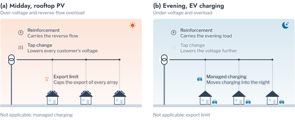
The mitigation measures of a distribution network act on different causes of violation. The voltage rise caused by rooftop Photovoltaic (PV) can be limited at its source by curtailing the active power of the inverters, through a volt-watt response or a static export limit [1], or by absorbing reactive power through a volt-VAr response [2]; AS/NZS 4777.2 requires both responses of every inverter in Australia. The voltage can also be lowered at the transformer by its off-circuit tap changer, which a field crew sets a few times a year rather than adjusting under load, so that a change of tap shifts the voltage of every customer at every hour. In terms of the voltage rise of Equation 7.1, the export limit and the volt-watt response reduce the injected power \(P_q\), the volt-VAr response sets \(Q_q\) against it, and the tap change lowers the sending voltage to which the rise is added. The evening violations caused by Electric Vehicle (EV) charging are relieved by moving the charging to the night [3]. Reinforcement, the replacement of a transformer by a larger one, relieves thermal violations at every hour. Figure 8.1 shows where each measure acts and which violations it relieves. A measure that relieves one violation can worsen another, since the tap change that lowers the midday voltage also lowers the evening voltage.
The choice among these measures has been formulated as an optimisation over a network model and as the reuse of past solutions. Xu and colleagues applied case-based reasoning to coordinated voltage control, retrieving the control actions that resolved similar past states of a distribution network with distributed generation and verifying them online before applying them [4]. The potential-outcome framework of Chapter 1 adds a consideration that case-based reasoning leaves implicit. A record of past measures is a log of the utility’s own decisions, in which a measure was applied where the problem appeared most severe, so that the outcomes that were not observed are missing not at random. Schnabel and colleagues treated recommendations as treatments and corrected both the evaluation and the training of recommenders on such logs by inverse-propensity weighting [5]. A mitigation measure also distributes a burden among customers, and the volt-watt response curtails the customers at the end of a feeder more than those near the transformer, because their voltage rises first; Liu and colleagues demonstrated this effect on the networks of AusNet and compared curtailment schemes by household measures of fairness [6], and Gerdroodbari and colleagues proposed a decentralised volt-watt control that distributes curtailment more equally among inverters [7]. During operation, finally, violations begin while others are in progress, and process industries treat the corresponding problem as the rationalisation of alarm floods, in which alarms are ranked by priority;1 Parvez and colleagues ranked alarm floods by their similarity to historical ones [8]. The sections of this chapter take up these four subjects in turn, beginning with what each measure does on HPK11.
Outcomes and Costs of the Mitigation Measures
The outcome of mitigation measure \(a\) on transformer \(j\) is the potential outcome \(Y_j(a)\), the hours of violation that remain under the measure, and its uplift is the number of hours it removes, Equation 6.19. Every measure was simulated on every transformer of HPK11 with popo, with PV and EVs at 80% of the residential customers and the AS/NZS 4777.2 inverter settings, and with the adopters, arrays and charging sessions drawn from the same seeded generator, so that the outcomes differ only by the measure. The measures are no action; a static export limit of 5 kW for every array; managed charging, which delays the evening charging of every vehicle to a start drawn between 22:00 and 02:00 while preserving its power profile; a change of the tap of every LV transformer by one step, which lowers its secondary voltage by approximately 2.5%; and the replacement of every LV transformer by the next standard rating. A further simulation without volt-watt response or export limit provides the generation that the measures curtail.
The measures acted on the violations that Figure 8.1 attributes to them (Table 8.1). The export limit reduced over-voltage from 1,675 to 1,269 transformer-hours and overload from 1,495 to 1,189, and curtailed 97.2 MWh of generation. The tap change reduced over-voltage to 634 hours and raised under-voltage from 75.5 to 371 hours. Managed charging reduced under-voltage to 64.5 hours and overload to 1,437.5. Reinforcement reduced overload to 735.5 hours and raised over-voltage by 9%, in both weeks, relieving the thermal constraint but not the voltage constraint; a larger transformer has a lower impedance and should reduce the voltage rise across it, and the source of this increase in the simulated network is examined with the seasonal simulation. The volt-watt response alone curtailed 2.0 MWh, and over-voltage was almost unchanged in its absence, at 1,678.5 hours.
A measure is chosen by its total cost, Equation 6.26: the annualised capital cost of the measure, the energy it curtails at a value \(\lambda\) per unit, and the violation that remains at a penalty \(\mu\) per hour. Absolute costs differ between utilities by an order of magnitude with the rating of the transformer,2 and the costs are therefore expressed relative to the annualised cost \(c_{\mathrm{r}}\) of reinforcing the transformer,
\[ \tilde C_j(a) = \frac{C_j(a)}{c_{\mathrm{r}}}, \tag{8.1}\]
with the results reported as functions of the ratios \(\lambda / c_{\mathrm{r}}\) and \(\mu / c_{\mathrm{r}}\). Here the capital costs relative to reinforcement are 0.05 for a tap change and 0.10 for managed charging, and curtailed energy is valued at 0.0002 per kWh. The penalty at which reinforcement becomes the measure of least cost for transformer \(j\) is its switching ratio,
\[ \mu_j^{\star} = \min \bigl\{ \mu : C_j(\mathrm{reinforcement}) \le \min_{a} C_j(a) \bigr\}, \tag{8.2}\]
the weight that a utility must give to a violation hour before it prefers investment to an operational measure.
The measure of least cost depended on the penalty assigned to a violation hour (Figure 8.2). No action was the measure of least cost for every transformer below a penalty of 0.0009 reinforcement annuities per violation hour, and the tap change for 98% of the transformers at 0.01. Reinforcement became the measure of least cost for 12 of the 43 transformers within the range examined, and for 28% at a penalty of one annuity per hour, at which the tap change remained the measure of least cost for 60% and the export limit for 9%. Managed charging was not the measure of least cost for any transformer in these two weeks, in which evening under-voltage amounted to 75.5 transformer-hours against 1,675 hours of over-voltage. At the central penalty, the median of the switching ratios of the 12 transformers that have one, the tap change was the measure of least cost for 32 of the 43 transformers, reinforcement for 6, the export limit for 4 and no action for 1. A single measure for the whole network would therefore misallocate most transformers, which motivates a recommendation for each.
Recommending a Measure for Each Transformer
A recommendation must be made before the outcomes of every measure are known for a transformer, and the recommenders differ in what they draw on. Not every measure applies to every violation: with \(\mathcal{A}_{\kappa}\) the set of measures that relieve violations of kind \(\kappa\), given by Figure 8.1, the recommendation for a transformer whose violations are of kind \(\kappa\) is restricted to
\[ \hat a_j \in \mathcal{A}_{\kappa} \cup \{0\}. \tag{8.3}\]
The regime rule of Part 5 (Regimes of Violation) applies this restriction directly. It assigns each transformer the measure that relieves its dominant violation with no action: the export limit for over-voltage, managed charging for under-voltage and reinforcement for overload. The regime-cluster policy uses the same grouping as clusters in the sense of Chapter 2, and assigns each transformer the measure of least mean cost among the other transformers of its group, a recommendation learned within each cluster rather than fixed by a rule, as cluster-based collaborative filtering recommends to a user the items preferred by its cluster [9]. The case-based policy of Chapter 1 estimates the cost of every measure for a transformer as the mean cost on its five nearest transformers, described by their rating, customers, impedance, demand and hours of each violation with no action, and selects the least.
Three recommenders learn instead from a field record, generated as in Chapter 1 by a utility that applied reinforcement with a probability rising from 0.15 to 0.85 with the overload of the transformer and an operational measure otherwise, and redrawn 200 times. The T-learner of Chapter 1 fits, for each measure, a regression of the cost on the features of the transformers that received it. Matrix factorisation, the principal method of collaborative filtering, estimates the missing entries of a matrix of users and items from its observed entries [10]. With transformers as users and measures as items, it estimates the cost of transformer \(j\) under measure \(a\) as
\[ \hat C_{ja} = m + p_j + q_a + \mathbf{u}_j^{\top} \mathbf{v}_a, \tag{8.4}\]
with a global mean \(m\), a baseline \(p_j\) for the transformer and \(q_a\) for the measure, and latent factors \(\mathbf{u}_j\) and \(\mathbf{v}_a\). It is fitted on the observed entries \(\mathcal{O}\) of the record, without weights and, in a second variant, with each entry weighted by the inverse of the propensity with which the utility selected that measure for that transformer [5],
\[ \min \sum_{(j, a) \in \mathcal{O}} \frac{\bigl( C_{ja} - \hat C_{ja} \bigr)^2}{\rho_a(\mathbf{x}_j)} + \gamma \bigl( p_j^2 + q_a^2 + \lVert \mathbf{u}_j \rVert^2 + \lVert \mathbf{v}_a \rVert^2 \bigr). \tag{8.5}\]
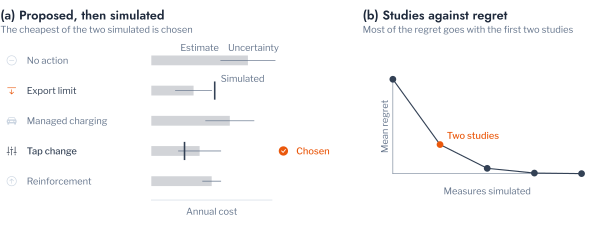
The last recommender verifies its proposals before it decides. Reasoning models in machine learning improve their answers by generating several candidates and retaining the one that a verifier scores highest, with a gain that grows with the number of candidates examined [11]. A utility can apply the same principle with its network model: the \(N\) measures of least estimated cost are simulated, and the measure of least simulated cost among them is selected,
\[ \hat a_j^{(N)} = \arg\min_{a \in \mathcal{T}_N(j)} C_j(a), \tag{8.6}\]
where \(\mathcal{T}_N(j)\) is the set of the \(N\) measures of least case-based estimate for transformer \(j\). Its regret, Equation 6.27, decreases to zero as \(N\) reaches the number of measures (Figure 8.3). Every recommender is evaluated at the central penalty by its mean regret, in units of the reinforcement annuity, and by the share of transformers to which it assigns the measure of least cost.
The recommenders differed by an order of magnitude in regret (Table 8.2). The regime rule assigned the measure of least cost to 16.3% of the transformers, with a mean regret of 1.87 reinforcement annuities, because it assigns the export limit to over-voltage, which the tap change relieves at lower cost on this network. The regime-cluster policy, which uses the same grouping but learns the measure within each group, assigned the measure of least cost to 74.4% of the transformers, with a mean regret of 0.21, the lowest of the recommenders that do not simulate. The regimes of Part 5 therefore identify the groups of transformers correctly, and the error of the rule lies in the measure it fixes for each group. The case-based policy assigned the measure of least cost to 69.8% of the transformers, with a mean regret of 0.26. The T-learner, fitted on field records in which reinforcement was applied where the overload was most severe, reached 42.4%, with a mean regret of 1.35.
Matrix factorisation did not exploit the field record. With one observed measure for each transformer, the baseline of the transformer absorbs its single entry, the latent factors of Equation 8.4 are not identified, and the fitted model assigns every transformer the measure of least mean cost in the record, which was the measure of least cost for 48.3% of the transformers. Weighting by inverse propensity, Equation 8.5, corrects the mean for the utility’s selection but not for the absence of entries, and reached 45.6%. Collaborative filtering therefore requires several measures recorded for each transformer, a condition that field records seldom satisfy.
Verification removed most of the regret that remained after the case-based estimate. Simulating the two measures of least case-based estimate and selecting the one of least simulated cost assigned the measure of least cost to 90.7% of the transformers and reduced the mean regret from 0.26 to 0.04; three studies assigned it to 97.7%. Two or three studies for each transformer thus recover nearly the full value of studying every measure, with the case-based estimate serving to select which measures to study. The measure of least cost, however, need not be the measure that treats customers equally, which the next section examines.
Equity of Curtailment
The burden of a measure on customer \(i\) is the share of the customer’s generation that it curtails,
where \(E_i^{\mathrm{f}}\) is the energy generated by the customer’s array without volt-watt response or export limit and \(E_i(a)\) the energy generated under measure \(a\). The inequality of the burden across the \(n\) customers of a network is measured by the Gini coefficient of Equation 6.28 and by Jain’s index,
\[ J(\mathbf{b}) = \frac{\bigl( \sum_{i} b_i \bigr)^2}{n \sum_{i} b_i^2}, \tag{8.8}\]
which equals one when the burden is shared equally and \(1/n\) when a single customer bears all of it [6]. Figure 8.4 contrasts the two forms of curtailment on a stylised feeder: the volt-watt response curtails the customers farthest from the transformer, and a static export limit curtails every array alike.
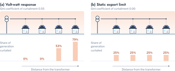
On HPK11 the curtailment was distributed unequally among customers (Table 8.3). Without any measure, the volt-watt response required by the inverter standard curtailed 0.08% of the generation of the average customer, a small burden but a concentrated one, with a Gini coefficient of 0.90 and a Jain’s index of 0.06. It fell on the customers at the highest impedance, from less than 0.01% in the two nearest quintiles to 0.27% in the farthest (Figure 8.5), in agreement with the findings of Liu and colleagues on other AusNet networks [6]. The export limit curtailed 3.2% of the generation of the average customer and distributed it evenly across positions, between 3.0% and 3.4% in every quintile of impedance. Its burden was nonetheless unequal, with a Gini coefficient of 0.79, because a static limit of 5 kW curtails only the arrays whose output exceeds the limit, and it therefore transfers the burden from the customers far from the transformer to the customers with large arrays.
Across the demand clusters of Part 5 the curtailment was nearly even, between 3.1% and 3.3% of generation under the export limit and between 0.07% and 0.10% with no action, consistent with the finding of Chapter 2 that the outcomes set by position are independent of the clusters of household demand. The export limit was modelled as a limit on the output of each array rather than on its net export, so the curtailment of households with high daytime demand is overstated. The burden of a measure is thus set by where a customer is connected and by the size of its array, and an equitable programme must be designed against these two quantities rather than against the type of household.
Ranking Live Violations for Operators
The recommendations of the preceding sections are made in planning, before the violations they address occur. During operation, violations begin while others are in progress, and an operator must determine which to address first. This is a ranking problem in the sense of Chapter 1. Each day of each penetration scenario of DSS-AU is a query in the query-level framework of learning to rank [12], and its list contains the violation events of that day, each represented as it is observed one hour after it began: its excess in its first two half-hours, its kind, the time and season of its start, the penetration scenario, and the rating and customers of its transformer. The relevance of an event is its final severity, the excess integral \(I_e\) of Part 5, which is unknown when the event is ranked (Figure 8.6). Events that end within their first hour are complete before they can be ranked and are excluded.
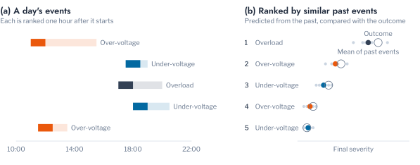
An event \(e\) is scored by the mean logarithmic severity of the \(k = 20\) past events nearest to it in the standardised features observed at one hour,
\[ \hat s_e = \frac{1}{k} \sum_{e' \in \mathcal{N}_k(e)} \log \bigl( 1 + I_{e'} \bigr), \tag{8.9}\]
which is the retrieval of Equation 6.3 applied to events, and by gradient-boosted trees fitted to the same target. Both are pointwise scores in the sense of Chapter 1, which order the events of a day through an estimate of the severity of each, and Equation 7.24 bounds the error of the ranking by the error of that estimate. Both are compared with the two quantities that an operator observes without a model, the current excess and the severity accumulated so far, and with a random order. The past events are those of the first half of each month and the days ranked those of the second half, so that no day contributes to both and events of the same day cannot inform one another, a form of leakage that would inflate the measured accuracy [13]. Each ranking is evaluated by the NDCG at 5 of Equation 6.14, the precision at 5 of Equation 6.11, and the share of the violation hours still to come that the five events ranked first account for, averaged over the days, with intervals from 500 bootstrap resamples of the days.
Scores learned from past events ranked the violations of each day more accurately than the quantities an operator observes directly (Figure 8.7). Over 2,331 days and 96,202 events, the gradient-boosted trees reached an NDCG at 5 of 0.962 and placed 81.0% of the five most severe events of a day among their first five, against 0.931 and 67.7% for the current excess and 0.916 and 62.1% for the severity so far. The nearest past events of Equation 8.9 reached 0.933 and 74.2%. The five events ranked first by the gradient-boosted trees accounted for 94.8% of the violation hours still to come among the five most severe events, against 86.1% for the current excess. On a typical day, an operator who attends first to the five events ranked highest by the model therefore attends to one more of the five most severe events than the current excess indicates.
Conclusion
This chapter recommended mitigation measures for the transformers of HPK11 from the simulated outcome of every measure on every transformer, and ranked violations during operation. The measures acted on the violations that their physics predicts: the export limit and the tap change on over-voltage, managed charging on evening under-voltage and reinforcement on overload, with the tap change worsening under-voltage. With costs expressed relative to reinforcement, the measure of least cost depended on the penalty assigned to a violation hour, and reinforcement became the measure of least cost for 12 of the 43 transformers.
The recommenders differed by an order of magnitude in regret. The regime rule of Part 5 assigned the measure of least cost to 16.3% of the transformers, because it does not consider the tap change, whereas a policy that learns the measure within each regime assigned it to 74.4%, so that the regimes of Part 5 serve recommendation as groups rather than as a fixed mapping; the case-based policy assigned it to 69.8%; and the simulation of the two measures of least case-based estimate assigned it to 90.7%, with a mean regret of 0.04 reinforcement annuities. Learners fitted on biased field records reached 42.4%, and matrix factorisation, with one measure recorded for each transformer, reduced to the assignment of the measure of least mean cost. The curtailment of the volt-watt response was small but fell on the customers of highest impedance, whereas a static export limit distributed it across positions and onto the customers with large arrays; across the demand clusters of Part 5 it was nearly even. Violations ranked one hour after they began were ordered more accurately by models of past events than by the quantities an operator observes directly, with a precision at 5 of 0.81 against 0.68.
The results on recommendation and equity rest on one January week and one July week at 80% adoption and on relative costs. The simulation of four seasonal weeks at 60% and 80% adoption will establish whether they hold across the year and at a lower adoption, in particular for managed charging, whose evening violations were few in both weeks. The field records are generated by a stated policy, and the recommenders have not been evaluated on the records of an operating network. The increase of over-voltage under reinforcement contradicts the expected effect of a lower transformer impedance and persisted in both weeks and is examined with the seasonal simulation before it is interpreted. Part 7 turns from violations that the simulator predicts to the detection of anomalous behaviour in measured data.
Exercises
- Increase the number of nearest past events in Equation 8.9 from 20 to 100. How do the NDCG at 5 and the precision at 5 of Figure 8.7 change, and why does a larger neighbourhood favour the long midday events over the brief evening ones?
- Rank the live events after their first half-hour rather than their first hour. What share of the advantage of the learned scores over the current excess remains?
- Raise the capital cost of managed charging in the
costscell from 0.10 to 0.30 reinforcement annuities. For how many transformers does the measure of least cost change at the central penalty?
References
The standards ANSI/ISA-18.2 and EEMUA 191 recommend that approximately 5% of alarms be of high priority, 15% of medium priority and 80% of low priority.↩︎
The Australian Energy Regulator publishes the value of curtailed exports as the customer export curtailment value, estimated half-hourly by region, and the unit rates of distribution transformers in the regulatory proposals of each network, in which the cost of a pole-mounted transformer of 25 kVA is approximately an order of magnitude below that of a kiosk of 500 kVA.↩︎