Segmentation for Network Studies
Chapter 4 located the weakness of the shape archetypes in their input rather than in the clustering. The archetypes describe when a household consumes, whereas the thermal risk of a transformer depends on how much its customers draw, and peak normalisation removes exactly that quantity. This finding raises three questions for the uses of segmentation in network operation. The first is whether the same pipeline, applied to an input that retains the level of demand, produces segments that retain the risk. The second is whether representative profiles drawn from such segments can replace the measured readings of every customer in a network study. The third is whether the identity of the customers who adopt Photovoltaic (PV) or an Electric Vehicle (EV) charger, described by these segments, changes the response of the network.
Segmentations that Retain the Level of Demand
The weakness of the archetypes thus lies in their input rather than in the clustering, which suggests that the same pipeline, applied to an input that retains the level of demand, should capture the risk that the archetypes miss. This section tests that proposition with three alternatives to the peak-normalised profile. The first appends three magnitude features, the logarithms of mean and peak demand and the load factor, to the normalised profile, with both blocks standardised and given equal weight. The second clusters the seasonal daily profiles in kW, so that level and timing enter together. The third describes each household by its coincident demand, its mean demand during the violations of each of the three extreme scenarios and the ratio of that demand to its usual demand at the same hour. Each input passes through the pipeline of the archetypes, a t-SNE embedding clustered with k-means. Every segmentation is compared at the \(K = 3\) of the archetypes, which is also the number of groups of the tercile reference, so that differences in the variance explained do not arise from different numbers of groups; Figure 5.2 compares every \(K\) from 2 to 12.
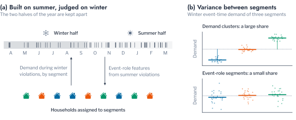
A segmentation fitted on the violations it is asked to explain would explain them by construction. The coincident-demand features are therefore computed from the violations of the summer half-year only, from October to March, and every segmentation is evaluated on household demand during the violations of the winter half-year, which none of them saw, together with the simulated outcomes of Attribution of Risk to Archetypes averaged over the customers assigned each household’s profile. The terciles of annual demand serve as a reference that requires no clustering. Figure 5.1 illustrates the design.
Table 5.1 reports the comparison, each share computed with Equation 4.4. The clustering of profiles in kW reached a silhouette of 0.516 and a balance of 0.995, better separated than the archetypes at 0.404. Its three segments explained 53.9% of the variance of winter demand during over-voltage, 44.8% during under-voltage and 41.0% during overload, against 13.6%, 5.7% and 4.8% for the archetypes, and 18.8% of the contribution to the network peak against 6.8%. Shape and size together explained 33.6 to 45.8% of the winter event-time demand. The demand clusters matched the terciles of annual demand, which explained 53.6%, 45.4% and 42.1%, so that clustering in kW recovers the level of demand without being given it as a feature. No segmentation explained more than 0.7% of the worst voltage, which confirms that voltage risk under PV resides in the point of connection rather than in the household.
The coincident-demand segmentation illustrates the hazard against which the held-out evaluation guards. It explained 39.6% of the contribution to the peak on a summer evening, more than any other segmentation, but only 7.8 to 9.5% of the winter event-time demand, because the summer violations from which it was built describe one season’s evening peaks rather than a persistent property of the household. A segmentation derived from network outcomes thus requires the same out-of-sample evaluation as a forecast before it can inform a decision.
This ranking held at every number of clusters (Figure 5.2). For winter demand during under-voltage, the demand-profile segmentation rose from 39.2% at \(K = 2\) to 64.0% at \(K = 10\), whereas the shape archetypes reached at most 15.3% for any \(K\) up to 12. For the contribution to the peak, the coincident-demand segmentation led at every \(K\), reaching 59.3% at \(K = 11\), consistent with the season of its construction, and the demand-profile segmentation rose to 31.1% at \(K = 12\), against at most 11.8% for the archetypes.
The three demand clusters are ordered by level (Table 5.2, Figure 5.3). Their mean demand is 0.27, 0.44 and 0.81 kW and their demand between 17:00 and 20:00 is 0.42, 0.69 and 1.26 kW, a threefold range, while all three share the evening peak of the archetypes. The demand clusters therefore cut across the archetypes rather than replacing them. The most peaked Archetype 1 makes up 63% of the lowest cluster and 15% of the highest, whereas the flattest Archetype 3 makes up 20% and 43%, so that a flatter use of the day is partly a property of larger households, yet every cluster contains all three archetypes.
Representative Profiles in Network Simulation
The preceding section measured how much of the risk a segmentation explains; network planning uses segmentations more directly. Planning studies seldom simulate the measured readings of every customer. They assign each customer a typical profile, often scaled to its billed consumption, and the accuracy of the study depends on how well the typical profiles stand in for the individual ones. This use therefore offers the most direct test of what a segmentation contributes to network analysis. HPK11 is simulated over the four seasonal weeks with random adoption of PV or EV chargers by 20 to 80% of customers, once with the measured readings and once with each of five sets of representative profiles. For a grouping \(g\) of the households, with \(g(i)\) the group of household \(i\) and \(E_i = \sum_t x_{i,t}\) its consumption over the year, the representative and scaled representative readings are
\[ r_{i,t} = \frac{1}{\lvert g(i) \rvert} \sum_{j \in g(i)} x_{j,t}, \qquad \tilde{r}_{i,t} = E_i \, \frac{1}{\lvert g(i) \rvert} \sum_{j \in g(i)} \frac{x_{j,t}}{E_j}, \tag{5.1}\]
so that the scaled profile keeps the shape of the group and restores the level of the household. The five sets are a single average profile for every household (one group), the mean profile of the household’s archetype, the same scaled, the mean profile of its demand cluster, and the same scaled. The adopters, array sizes and charging sessions are identical in every run, so that differences in outcome arise from the household profiles alone.
Table 5.3 compares the outcomes with those of the simulation with measured profiles, both as time series and as events. For a series \(y\) such as the loading of a transformer, with \(\hat{y}\) its value under representative profiles, the error is the root-mean-square difference over all transformers \(j\) and half-hours \(t\) of the simulated weeks; the violation hours are compared by the ratio of totals over the transformers; and the classification is compared by the share of transformers, levels and constraints on which the two simulations agree about the criterion of Equation 4.1, applied to the simulated period:
\[ \text{RMSE} = \sqrt{\frac{1}{\lvert \Omega \rvert} \sum_{(j, t) \in \Omega} (\hat{y}_{j,t} - y_{j,t})^2}, \qquad R = \frac{\sum_j \hat{D}_j}{\sum_j D_j}, \qquad A = \frac{1}{\lvert \mathcal{J} \rvert} \sum_{\mathcal{J}} \mathbb{1}\left[ \mathbb{1}[\hat{D}_j \le \theta] = \mathbb{1}[D_j \le \theta] \right], \tag{5.2}\]
where \(\Omega\) is the set of transformer half-hours, \(\mathcal{J}\) the set of transformer, level and constraint combinations, and \(\theta\) 1% of the 672 simulated hours. As time series, every set of representative profiles reproduced the loading of the transformers closely, with a root-mean-square error between 0.020 and 0.022 pu, and the lowest customer voltage within 5.7 to 6.8 thousandths of a per unit. The demand clusters reduced each error relative to the single average profile, and scaling to each household’s consumption reduced it further, to 0.0197 pu of loading and 5.70 thousandths of lowest voltage for the scaled demand clusters.
As events, the representative profiles differed markedly (Figure 5.4). The midday regimes were reproduced within 8%, with ratios \(R\) of over-voltage hours to the simulation with measured profiles between 0.925 and 0.949 and of PV-driven overload between 0.995 and 1.013. EV-driven under-voltage, the brief evening regime, was underestimated by every set: the single average profile produced 58.8% of the measured hours, the archetypes 61.1%, the demand clusters 67.1%, the scaled demand clusters 79.9% and the scaled archetypes 92.9%. Without Distributed Energy Resources (DER) the measured readings produced 14.0 hours of under-voltage over the four weeks, which the unscaled representatives reduced to at most 1.0 hour.
The difference lies in what averaging removes. A representative profile is the mean of about a hundred households and is therefore smooth, whereas an evening under-voltage occurs when the peaks of many customers on one feeder coincide. Retaining the level of demand, through clusters in kW or through scaling to each household’s consumption, restores the spread of demand across customers and recovers part of the under-voltage, but the diversity of timing within a cluster is lost in every case (Figure 5.5). The two segmentations are complementary in this use. Where only profiles are available, the demand clusters reproduced the evening regime better than the archetypes or a single average, and where billed consumption supplies the level of each customer, the scaled shape archetypes reproduced it most closely. On the classification that informs hosting decisions, whether a transformer remains within the criterion of violations in at most 1% of the time, all sets agreed with the simulation with measured profiles in 96.0 to 97.2% of cases.
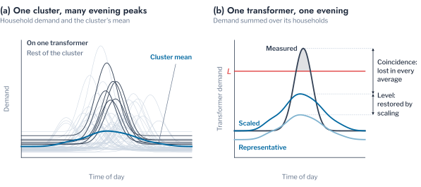
Figure 5.6 shows this loss on the evening of lowest voltage in the simulated weeks, 16 January, with EV chargers at 80% of customers. Every set of representative profiles reproduced the timing of the evening and the loading of the transformer, which peaked at 1.35 to 1.39 times its rating against 1.38 for the measured readings, and every set breached the lower voltage limit. The measured readings, however, reached a lowest voltage of 0.841 pu, against 0.863 to 0.884 pu for the representative profiles, so that the representatives reproduce the occurrence of the violation but underestimate its depth.
Effect of Who Adopts
In every analysis so far, including the simulations of the preceding section, the adopters are fixed by a random draw, as in DSS-AU. Adoption in practice is neither random nor uniform, since it varies between areas with their building stock and socio-economic characteristics [5], and segments offer a natural means of describing who adopts. This section therefore holds the number of installations fixed and varies their allocation. For adoption by a share \(\ell\) of the \(N\) residential customers, from 10 to 25%, the \(n = \ell N\) adopters are drawn without replacement from an eligible set \(\mathcal{S}\): all customers for a random allocation, the customers of one archetype or of one demand cluster for a segment allocation, and, for a concentrated allocation, the customers of whole transformers taken in a random order until \(\lvert \mathcal{S} \rvert \ge n\), of whom the first \(n\) adopt, so that every chosen transformer but the last is fully equipped (Figure 5.7). The level of 25% is the largest that the smallest segment, with 1,514 customers, can supply. Each allocation is solved over the four seasonal weeks with two seeds.
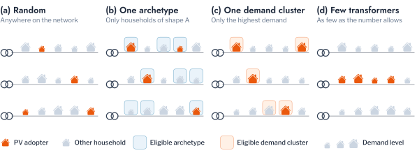
The geographical concentration of adoption changed the network response more than any behavioural allocation (Figure 5.8, Table 5.4). With PV at 25% of customers, random placement produced 1,515.5 hours of over-voltage on 40 transformers and 9.8 hours of overload on 3 transformers. Concentrated placement reduced the over-voltage to 1,298.0 hours, because it reached only 10.5 transformers on average, but raised the overload to 1,119.0 hours on 14.5 transformers. Concentrated EV adoption likewise raised under-voltage from 59.2 to 91.2 hours and overload from 90.8 to 115.0 hours, although the range between seeds of 70.5 to 159.5 hours for overload indicates that the effect depends on which transformers receive the chargers.
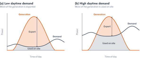
Among the behavioural allocations, the demand clusters separated the outcomes far more than the archetypes. PV installed only by the households of the highest-demand cluster produced 1,206.2 hours of over-voltage, 20.4% less than random placement, whereas PV installed only by the lowest-demand cluster produced 1,794.8 hours, 18.4% more. The three archetypes spanned 1,405.8 to 1,579.0 hours, a range of 173.2 hours against 588.6 hours across the demand clusters. The direction agrees with the event-time demand of Demand at the Time of Violation, since households with a larger midday demand consume more of their own generation and export less of it (Figure 5.9). For EVs the allocation by segment made no consistent difference to overload, which ranged from 88.5 to 91.8 hours across the random and segment allocations, and only a modest one to under-voltage, from 56.5 to 73.0 hours, against a range between seeds of 51.0 to 67.5 hours under random placement.
Implications for Network Operation
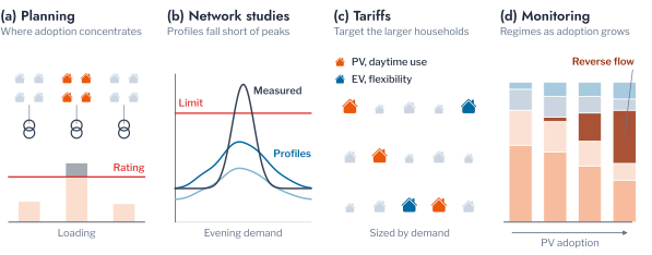
Taken together, the results bear on four activities of a Distribution System Operator (DSO), summarised in Figure 5.10. For connection assessment and reinforcement planning, the exposure of a transformer was determined by its loading ratio and its number of customers, which correlated with overload and over-voltage hours at 0.943 and 0.743, and by the geographical concentration of adoption, which raised PV-driven overload at 25% adoption from 9.8 to 1,119.0 hours over four weeks. The regimes of violation add a temporal dimension to these decisions. On HPK11, reverse-flow overload is absent below 40% PV penetration and becomes the largest regime at 80%, so that an assessment made at a low penetration does not reveal the constraint that later adoption will impose.
For network studies that cannot use every customer’s readings, clustering supplies the representative profiles, and the choice of segmentation matters more for the evening regime than for the midday ones. Profiles that retained each customer’s level of demand, through clusters in kW or through scaling to billed consumption, recovered 67.1 to 92.9% of the EV-driven under-voltage hours, against 58.8% for a single average profile. Since every set of representatives underestimated the brief evening violations, studies of EV hosting based on typical profiles should be read as lower bounds on the duration of under-voltage.
For tariff design and customer engagement, segments defined by the level of demand identify the households that matter. Confining PV adoption to the highest-demand cluster reduced over-voltage by 20.4% relative to random placement, which suggests that combining PV with daytime consumption, for instance through time-of-use incentives or storage, is most effective when aimed at larger households. The demand present at evening violations likewise followed the level of household demand rather than its shape, so that flexibility programmes for EV-driven under-voltage should select customers by consumption and location rather than by profile shape.
For monitoring, two uses of clustering complement the time-series record. The regimes of violation summarise a year of events per transformer into a small number of recognisable types, whose shares indicate which remedy a transformer requires as penetration changes. The shape archetypes, although they carry little information about risk, remain useful for detecting new behaviour, since forty households given an EV charging profile formed a pure archetype of their own, displacing an existing archetype unless the number of archetypes was allowed to grow by one. This use requires that the clustering be repeated on a schedule and with at least a season of history.
Table 5.5 summarises which product of clustering serves each decision, and the evidence for it in this chapter and the last.
| Decision | Product of clustering | Evidence |
|---|---|---|
| Connection assessment and reinforcement | Regimes of violation per transformer | Reverse-flow overload absent below 40% PV and the largest regime at 80% (Regimes of Violation) |
| Network studies without every customer’s readings | Representative profiles that retain the level of demand | 67.1 to 92.9% of EV under-voltage hours recovered, against 58.8% for one average profile (Representative Profiles in Network Simulation) |
| Tariffs and engagement programmes | Demand clusters (segments of the level of demand) | 20.4% less over-voltage with PV in the highest-demand cluster (Effect of Who Adopts) |
| Flexibility programmes for EV charging | Annual demand and location, not profile shape | Event-time demand correlated with annual demand at 0.806 during under-voltage (Demand at the Time of Violation) |
| Monitoring of behaviour | Shape archetypes, recomputed with \(K + 1\) evaluated | EV charging formed a pure archetype, displacing an existing one at a fixed \(K\) (Chapter 3) |
Conclusion
This chapter evaluated three uses of segmentation in network operation. Applied to profiles in kW, the pipeline of Chapter 2 produced three demand clusters that explained 41.0 to 53.9% of the demand during the violations of a held-out half-year and 18.8% of the peak contribution, as much as the terciles of annual demand. A segmentation built from summer violations explained the summer peak contribution best but failed in winter, which shows that a segmentation derived from network outcomes requires out-of-sample evaluation. In network simulation, representative profiles that retained the level of demand reproduced the evening under-voltage better than a single average profile, although every set underestimated its depth. As allocations of adoption, the demand clusters separated the over-voltage outcome 3.4 times more widely than the archetypes, while the geographical concentration of adoption changed the response more than any behavioural allocation.
These conclusions are subject to several limitations. The households are placed on the network by a random draw, so the analysis cannot represent geographical clustering of behaviour, and the network is a single urban feeder with a pseudo LV topology. The direct simulations cover four weeks, one per season, with two seeds per configuration, and the attribution scenarios of Chapter 4 equip every customer, which isolates demand and location at the cost of realism. The regimes of violation are derived from one network and one year of weather, and all analyses use the demand of one population.
The results also define what the next chapter must address. The demand clusters reached only the explanatory power of a simple tercile of annual demand, and no segmentation approached the 69.6% of the peak contribution that the household itself explains. Representative profiles, moreover, lost the diversity of timing that produces brief evening violations. Chapter 6, in preparation, examines representations of a household that retain magnitude and describe its demand across several time scales, and asks whether the groupings they produce close the gap between segment and household.
Key findings
Segments that retain the level of demand captured the risk that shape archetypes miss: three demand clusters explained about half of the demand present during held-out violations. Representative profiles reproduced the midday regimes closely and the brief evening under-voltage only in part, best when they retained each customer’s level. Where adoption concentrated mattered more than which segment adopted, and among segments, the level of demand mattered more than its shape. A segmentation derived from network outcomes must be evaluated on outcomes it did not see.
Exercises
- In the
segmentationscell of the companion notebook, evaluate every segmentation at \(K = 5\) instead of the common \(K\). Does the ranking of Table 5.1 change? - Using the simulated records of the
replaycell, find the evening of lowest voltage under EV charging at 40% rather than 80%. Do the representative profiles still breach the lower limit on that evening? - Add to the
adoptioncell an allocation confined to the households with the highest demand at the half-hour of the network peak. How does it compare with the highest-demand cluster?