Customer Archetypes and Their Reliability
Chapter 2 settled a clustering pipeline on three metered populations and closed on a practice: every index is read together with the cluster sizes, the archetype curves and, where available, an external attribute. This chapter applies the pipeline and that practice to the 342 households of the AusNet population and asks whether the resulting archetypes are reliable enough to support decisions that persist.
Load-profile archetypes are routinely proposed as a basis for tariff design, demand response and network planning [1], [2], [3]. Each of these uses stores a household’s archetype and acts on it for months or years, and therefore rests on three properties that internal validity does not establish. The assignment of each household must be certain enough to act upon, the method that produces it must not be improved upon by a more elaborate one, and the assignment must persist for as long as the decision applies. Kwac, Flora and Rajagopal observed that the daily load shape of one household varies considerably from day to day [2], which suggests that the third property in particular cannot be assumed. Chapter 2 also showed that resampling evidence is comparable across the number of clusters only after calibration, so the choice of \(K\) itself is the first property to verify.
The chapter is organised as follows. Archetypes of the AusNet Population derives the archetypes and verifies the choice of \(K\) against calibrated resampling evidence. Reliability of the Archetypes examines the certainty of membership through conformal prediction, compares k-means with a consensus method, measures the persistence of the archetypes over a year, tests whether they register a controlled change in behaviour, and determines how much history they require. Conclusion concludes and leads to Chapter 4, which asks whether the archetypes carry information about network risk.
Archetypes of the AusNet Population
This section applies the pipeline of Chapter 2 without modification. Each household is represented by its peak-normalised seasonal profiles over the year, with the seasons defined for the southern hemisphere. The profiles are not scaled; they are embedded by t-SNE at a perplexity of thirty and clustered with k-means. Figure 3.1 shows how eight internal indices rate the number of clusters on this embedding. Five of them, density silhouette, Calinski-Harabasz, Davies-Bouldin, MMI and CVFLDA, prefer \(K = 2\), whereas the weighted Borda ranking of Chapter 2 recommends \(K = 11\), the value it also recommended on London.
The two recommendations differ in how well they reproduce. Chapter 2 showed that internal indices cannot settle a disagreement between partitions that all score well, and the first instrument it applied to such a disagreement is the trust-gated composite score of Equation 2.3. Table 3.1 lists its six highest-ranked values of \(K\). At \(K = 2\) the prediction strength was 0.917 and the smallest cluster-wise stability 0.970; at \(K = 3\) these fell to 0.748 and 0.884, and at \(K = 11\) to 0.297 and 0.479. The composite therefore ranked \(K = 2\) first, with a score of 0.970 against 0.593 for \(K = 3\).
The trust factor of this score, however, rests on uncalibrated resampling evidence, which Chapter 2 showed to favour a two-way split for structural reasons: on structureless data, prediction strength is high at \(K = 2\) and low at large \(K\). Following the practice of Chapter 2, the number of archetypes is therefore chosen from the calibrated excess of Equation 2.4, as the value with the largest mean excess among those whose excess is positive on every check,
\[ K^{*} = \arg\max_{K \in \mathcal{K}^{+}} \bar{\Delta}(K), \qquad \mathcal{K}^{+} = \{\, K : \Delta_m(K) > 0 \text{ for every check } m \,\}. \tag{3.1}\]
Only \(K = 2\) and \(K = 3\) had a positive excess on all three checks (Table 3.2). The excess at \(K = 2\) was small, at 0.020 for prediction strength, 0.009 for cluster-wise stability and 0.041 for subsample agreement, a mean of 0.023, whereas \(K = 3\) had the largest excess of any value, 0.118, 0.131 and 0.212, a mean of 0.154. The Borda value of 11 reproduced worse than the reference on all three checks, with a mean excess of \(-0.052\). The connectivity check of Chapter 2 found no isolated group: the nearest-neighbour graph of the embedding remained a single connected component from 10 to 100 neighbours, so the AusNet population contains no minority cohort of the kind found in London.
The calibrated evidence thus selects \(K = 3\). The two-way split that the composite preferred reproduces barely better than structureless data, which is the structural bias that Chapter 2 identified, while three archetypes reproduce substantially better. The remainder of the part uses \(K = 3\) and retains the composite’s \(K = 2\) and the Borda value of 11 as alternatives wherever the comparison is informative; Chapters 4 and 5 show that their conclusions about network risk do not depend on this choice.
The three archetypes contain 133, 101 and 108 households (Figure 3.2). All three peak in the early evening, at 19:00, and they differ in the demand that surrounds this peak. Archetype 1 is the most peaked: its mean profile falls to about 0.21 of the daily maximum before dawn and holds near 0.44 between 10:00 and 16:00, so that its evening peak stands well above the rest of the day. Archetype 2 has a pronounced morning peak of about 0.56 at 08:00 and a daytime level near 0.54. Archetype 3 is the flattest, with a base near 0.42 before dawn, a daytime level near 0.58 and a later, broader morning peak at about 09:30. The division is therefore between more and less peaked uses of the same evening, distinguished by the base load and the morning, rather than between households that are active at different times.
In the embedding the three archetypes divide one continuous cloud rather than three separated groups (Figure 3.3), which is consistent with a silhouette of 0.404. The algorithms of Chapter 2 confirm the division to different degrees (Table 3.3). A Gaussian mixture reproduced it closely, with an ARI (Equation 1.12) of 0.866 against k-means [4], and Ward linkage agreed at 0.646, with a balance of 0.973, because it placed the boundaries elsewhere in the same continuum. A division of a continuum, rather than a separation of distinct groups, raises the question of how reliably each household is assigned, which the next section examines.
Reliability of the Archetypes
A segmentation can support a decision only if the assignment of each household is certain, if a more elaborate method does not improve upon it, and if the assignment persists for as long as the decision applies. This section examines these three properties in turn, and then the ability of the archetypes to register a change in behaviour and the length of history they require.
Certainty of Membership
A partition assigns every household to one archetype, including households that lie near a boundary or far from every centre. Split conformal prediction replaces this single assignment with a set of archetypes that carries a coverage guarantee [5]. The clusterer is fitted on 70% of the households, and for each of the \(n = 103\) households held back, with embedding \(\mathbf{z}_i\), the distance to the nearest centroid is recorded as its score \(r_i = \min_k d(\mathbf{z}_i, \mathbf{c}_k)\). For a miscoverage level \(\alpha\), the threshold \(\hat q\) is the \(\lceil (n + 1)(1 - \alpha) \rceil\)-th smallest of these scores, and every household receives the set of archetypes whose centroids lie within it,
\[ \Gamma(i) = \{\, k : d(\mathbf{z}_i, \mathbf{c}_k) \le \hat q \,\}. \tag{3.2}\]
Provided the households are exchangeable, a new household’s nearest centroid lies within \(\hat q\), and its set is therefore not empty, with probability at least \(1 - \alpha\); here \(\alpha = 0.1\). A set of one archetype is a confident assignment, a set of two marks a household on the boundary, and an empty set marks a household that no archetype describes as well as the calibration households were described (Figure 3.4).
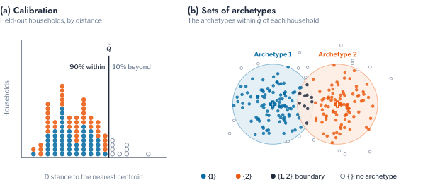
With a threshold of 9.321 embedding units, 273 of the 342 households (79.8%) received a single archetype, 49 (14.3%) a set of two and 20 (5.8%) an empty set (Table 3.4). The empty sets remained within the 10% that the miscoverage level \(\alpha\) allows. The two kinds of uncertain set identify different households: a set of two marks a household whose demand lies between two archetypes and could be assigned to either, and an empty set a household atypical of all three, which assumptions made at the level of the archetype describe least well. Together they account for one household in five.
Comparison with a Consensus Method
Uncertain membership could reflect a limitation of k-means rather than of the data. The literature on load-profile clustering repeatedly proposes more elaborate methods than k-means [1], [6], of which deep clustering is a current instance [7], [8]. A consensus over twenty k-means runs with different seeds rests on the same principle, that combining many partitions corrects the weaknesses of any one [9], at a fraction of the cost. Table 3.5 compares it with k-means for \(K\) from 2 to 8.
At \(K = 2\) and \(K = 3\) the consensus returned the k-means partition itself, with an ARI of 1.000 at the chosen \(K = 3\) and identical separation indices. At larger \(K\) it was no better and in places worse; at \(K = 5\) its silhouette was 0.334 against 0.366 and its Davies-Bouldin index 1.011 against 0.916. On an embedding on which k-means is already stable across seeds, combining seeds has nothing to correct, and the remaining question of reliability concerns time rather than method.
Stability over the Year
An archetype can inform a persistent decision, such as a tariff or a connection approval, only if the household retains it. Each quarter of the year is therefore clustered separately with the same pipeline at \(K = 3\), and the agreement between quarters is compared with the variation due to the algorithm alone, measured by runs on the same quarter with different seeds (Figure 3.5).
The separation within each quarter barely changed, with silhouettes between 0.375 and 0.418, and partitions of the same quarter with different seeds agreed perfectly. Partitions of different quarters, in contrast, agreed at an ARI of only 0.169 to 0.259. The difference is therefore behavioural rather than algorithmic: the population divides as cleanly in every quarter, but not along the same households. Because each quarter is clustered separately, its archetype numbers are arbitrary, and the archetypes of the first and last quarters are matched so as to maximise the number of households that keep theirs (Figure 3.6). Even under this most favourable matching, 136 of the 342 households (39.8%) changed archetype within the year.
Pitfall: treating an archetype as a fixed attribute
An archetype computed from one period describes that period. A label assigned from one quarter’s profile and stored as a customer attribute was wrong for two households in five by the end of the year, and nothing in the stored label indicates which. Archetypes that inform persistent decisions must be recomputed on a schedule, and the turnover between runs is itself a quantity to monitor.
Detection of a Change in Behaviour
The sensitivity to behaviour that limits the archetypes as a fixed attribute also makes them a candidate instrument for monitoring, since a group of households that changes its behaviour should be registered by a periodic re-clustering. This property is tested under controlled conditions. Forty households are chosen at random, 12, 15 and 13 from the three archetypes, and a diversified Level-2 charging profile, peaking at 1.49 kW per vehicle at 21:00, is added to every day of their year before the population is clustered again.
At the established \(K = 3\) the adopters were isolated: 39 of the 40 formed a cluster of their own, a recall of 0.975 and a purity of 1.000 by Equation 1.14 (Table 3.6). The new archetype displaced an existing one. The households of Archetype 1 remained together, those of Archetype 3 joined about half of Archetype 2, and the other half of Archetype 2 joined Archetype 1. With one more archetype the adopters remained isolated at the same recall and purity, and the remaining households were again divided into three groups (Figure 3.7). The adopters’ profile has an overnight trough near 0.13 of the daily maximum and an evening level near 0.82 between 21:00 and 23:30, later than in any original archetype. A change of this size therefore appears as an archetype of its own, but at a fixed \(K\) it does so by absorbing an existing archetype into its neighbours, which indicates that a monitoring schedule should evaluate \(K + 1\) alongside the established \(K\).
History Required
Both stability and monitoring depend on the length of the record that is clustered. Each clustering in this chapter uses a year of readings, whereas a utility clustering newly metered customers, or re-clustering on a schedule, must decide how much history suffices. Figure 3.8 clusters the mean daily shape of the first day, week, month and season of the year at \(K = 3\) and compares each partition with that of the first season.
A single day agreed with the season at an ARI of 0.008, a week at 0.160 and a month at 0.296. The silhouette rose with the window, from 0.116 for a day to 0.190 for the season, but a week was as well separated as a day, at 0.118, while agreeing with the season twenty times as closely, so that the silhouette of a short window says little about the households it describes. A month recovered less than a third of the seasonal structure, and a full season was required to reproduce it.
Conclusion
This chapter applied the pipeline of Chapter 2 to the AusNet population and assessed whether its archetypes can support decisions that persist. Calibrated resampling selected three archetypes, with a mean excess of 0.154 over a structureless reference, against a marginal 0.023 for the two-way split that the uncalibrated composite preferred and a negative excess for the eleven that the Borda ranking recommends. The three archetypes are more and less peaked uses of the same evening, distinguished by the base load and the morning, and divide one continuous cloud rather than separate three groups.
The reliability of the archetypes as a basis for persistent decisions proved limited. At the 90% conformal level, 14.3% of households lay between two archetypes and 5.8% fitted none. A consensus over twenty seeds returned the k-means partition itself, so the limitation lies in the data rather than in the method. Between the first and last quarters, 39.8% of households changed archetype under the most favourable matching, and a season of history was the minimum that reproduced the division. The archetypes did register a controlled change in behaviour: forty households given an evening charging profile formed an archetype of their own, at the cost of merging the intermediate archetype into its neighbours.
An archetype is therefore a property of a period rather than of a household, useful for monitoring change but unsafe as a stored attribute. These results describe the archetypes on their own terms; they do not establish whether the archetypes bear on the risks that motivate their use. Chapter 4 places the same households on a real network and answers that question.
Key findings
Calibrated resampling selected three archetypes in the AusNet population, which differ in the shape of the same evening; the uncalibrated composite preferred two, a split that reproduces barely better than structureless data. One household in five received an uncertain conformal set, two in five changed archetype within a year, and a full season of history was needed to reproduce the division. Archetypes should be recomputed on a schedule, with \(K + 1\) evaluated alongside \(K\), rather than stored as customer attributes.
Exercises
- Run the calibration in the
pipelinecell of the companion notebook with four times as many reference draws and resamples. How much do the excesses at \(K = 2\) and \(K = 3\) move, and does either change sign? - Change the miscoverage level \(\alpha\) of the
conformalcell from 0.1 to 0.2 and to 0.05. How do the shares of empty sets and of sets of two follow \(\alpha\)? - Repeat the
quartersanalysis with months instead of quarters. Does the share of households that change archetype grow, and how does the agreement between consecutive months compare with that between consecutive quarters?