Clustering for Network Risk
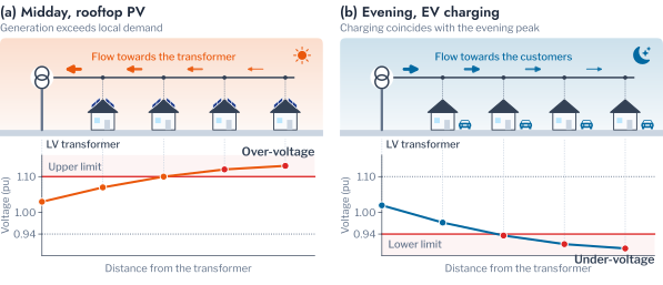
The operation of a Low Voltage (LV) network is bounded by two kinds of constraint: the voltage at every customer must remain within a statutory band, and the loading of every transformer must remain within its rating. Rooftop Photovoltaic (PV) and Electric Vehicle (EV) charging act on both, in opposite directions (Figure 4.1). Midday export from PV raises voltages and, where it exceeds local demand by a wide margin, reverses the flow through the transformer and overloads it, whereas evening charging adds demand at the hour of the daily peak and depresses voltages at the ends of long feeders. A Distribution System Operator (DSO) that must decide where to reinforce, which connection requests to approve and which customers to engage in a tariff or flexibility programme therefore needs to know how these violations develop as adoption grows, when they occur, and which customers are associated with them [1], [2].
Chapter 3 derived archetypes from the AusNet population and found them reproducible within a period but not permanent across periods. Archetypes of this kind are proposed as the basis for exactly the decisions above, on the premise that households which use energy at similar times affect the network in similar ways. Reliability does not establish that premise, and this chapter tests it on a real network. In doing so it applies clustering to both kinds of data that a DSO holds: the smart-meter time series of its customers and the record of limit violations on its transformers. The test is possible because the 342 AusNet households form the demand pool of four AusNet Medium Voltage (MV)-LV network models published by the University of Melbourne,1 so that the households that are clustered can also be placed on a network model and simulated. Of these networks, the urban network HPK11 supplies 5,274 residential customers from 43 of its 44 LV transformers, and the DSS-AU dataset records every half-hour of a year on it under 25 combinations of PV and EV penetration.
Related Work
The established frame for assessing Distributed Energy Resources (DER) on distribution networks is hosting capacity, the amount of generation or demand a network can accommodate before a performance index, such as the time a voltage spends outside its band, exceeds its limit [3], [4]. Because the outcome depends on which customers adopt and on what they consume, probabilistic impact assessments sample household demand profiles and the locations of adoption, and report the share of feeders that remain within their limits as penetration grows [5], while recent work estimates hosting capacity from data rather than from repeated power-flow studies [1], [2]. The remedies differ by constraint: over-voltage from PV export is addressed by curtailment of active power or by reactive power control in the inverter [6], [7], whereas the overload and under-voltage of EV charging are addressed by coordinating when vehicles charge [8].
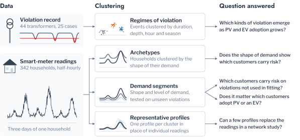
Two gaps follow for the use of clustering. Hosting studies summarise violations as shares of time or of feeders within limits, which do not distinguish a long midday excursion from many brief evening ones, although the two call for different remedies. Load-profile segmentation, for its part, has been assessed by internal indices and by the correspondence of its clusters with household characteristics [9], [10], [11], and seldom by the network outcomes it is proposed to inform. This chapter addresses both gaps: it clusters the violations themselves into regimes, and it measures how much of the risk of each customer its archetype carries. Chapter 5 then evaluates the uses of clustering that the result points to. Figure 4.2 summarises the products of clustering in the two chapters and the operational question that each serves.
The remainder of the chapter is organised as follows. Network, Data and Violation Events describes the network model, the simulations and the definition of a violation event. Network Response to DER Penetration characterises the response of the network to DER penetration and Regimes of Violation clusters the violations into regimes. Demand at the Time of Violation examines household demand at the moments of violation, Attribution of Risk to Archetypes decomposes per-customer risk, and Conclusion concludes.
Network, Data and Violation Events
The network analyses use HPK11, the urban network of Hampton Park, Victoria. Its definition is rebuilt from the published workbook as an OpenDSS model of the 22 kV feeder and the 44 LV transformers of 200 to 1,000 kVA beneath it, with a pseudo LV network extending to every customer. One of these transformers supplies no residential customer and records no customer voltage, so the analyses at the level of the transformer concern the other 43. Each of the 5,274 residential customers is assigned the measured load profile of one of the 342 AusNet households, drawn with replacement under a fixed seed, so that each household appears at about fifteen locations and the archetype of every customer is known.
Two sources of network outcomes are used. The DSS-AU dataset, computed with popo on this model, records every half-hour of 2019 for each LV transformer under 25 scenarios, in which PV and EV penetration each range from 0 to 80% of customers in steps of 20. Arrays of \(6.6 \pm 2.0\) kWp follow measured irradiance with temperature derating and the AS/NZS 4777.2 volt-VAr characteristic, and chargers follow recorded charging sessions. Each record holds the loading of the transformer relative to its rating and the lowest and highest voltage among its own customers. Where a question requires control over which customers adopt, or over the load profile assigned to each customer, the same model is solved directly with popo over four weeks, one in each season, beginning on 11 January, 11 April, 10 July and 10 October, with the same inverter settings.
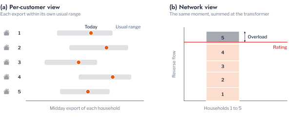
Outcomes are recorded at the transformer rather than at each customer because a violation arises from the coincidence of ordinary demands on one transformer. Figure 4.3 illustrates this for export: the midday export of each household lies within its own usual range, and only their sum at the transformer exceeds the rating.
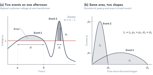
Even at the level of the transformer, a record of 19.3 million half-hours requires a summary. A share of half-hours beyond a limit indicates how often the limit is breached, but not whether the breaches form one long afternoon or many brief excursions, which call for different remedies. The record is therefore summarised as events. For a series \(x_t\) at a transformer and a limit \(L\), the excess is \(e_t = x_t - L\) for an upper limit and \(e_t = L - x_t\) for a lower one. An event is a maximal run of consecutive steps \(a \le t \le b\) with \(e_t > 0\), characterised by its duration \(d = (b - a + 1)\,\Delta\), its peak excess \(\max_t e_t\) and its integral \(I = \Delta \sum_{t=a}^{b} e_t\), where \(\Delta\) is half an hour; the integral weighs depth and duration together. Four kinds of event are extracted. Over-voltage and under-voltage occur when the highest or lowest customer voltage leaves the AS 61000.3.100 band of 0.94 to 1.10 pu, overload when the apparent power exceeds the nameplate rating, and high loading when it exceeds 90% of the rating, the early warning of an overload. The year yielded 292,041 events across the 25 scenarios. Figure 4.4 illustrates the definition and shows why duration, peak excess and integral are all required, since a long, shallow event and a brief, deep one can enclose the same area.
Network Response to DER Penetration
With violations defined as events, the response of the network to DER can be described in terms that bear directly on decisions. This section characterises how violations develop as penetration grows, which transformers reach their limits first, when the violations occur, and which properties of a transformer determine its exposure.
Frequency, Duration and Depth of Violations
Figure 4.5 shows the total duration of each kind of violation across the 25 scenarios. The two technologies stressed the network along different constraints. Over-voltage depended almost entirely on PV: it was absent without PV, reached 8,791 hours at 20% PV and rose to 46,546 hours at 80%, with EV adoption reducing it only slightly. Under-voltage depended on EV adoption, rising from 22 hours without DER to 1,044 hours at 80% EV, and PV reduced it moderately, to 797 hours at 80% of both. Overload responded to both technologies but on different scales. EV charging at 80% produced 923 hours, whereas PV at 60% already produced 8,339 hours and at 80% 29,088 hours, so that reverse power flow dominates the thermal exposure of this network.
The events also differed in character (Table 4.1). With PV at 80%, over-voltage events lasted 4.01 hours on average and up to 9.00 hours but rose at most 0.05 pu above the limit, while overloads lasted 4.14 hours on average and reached 1.15 pu beyond the rating, a loading of 2.15 times nameplate. With EVs at 80%, events were shorter, with mean durations of 1.19 hours for under-voltage and 1.63 hours for overload; under-voltage reached 0.09 pu below the band and overload 0.69 pu beyond the rating. PV-driven violations are thus long and shallow in voltage but deep in loading, whereas EV-driven violations are brief excursions concentrated around the evening peak.
Hosting Thresholds
These totals aggregate over transformers that differ widely in their exposure. A transformer \(j\) is taken to host a penetration level when the total duration of its violations of a limit over the year, the sum \(D_j = \sum d\) over its events of that kind, satisfies
\[ D_j \le 0.01 \times 8{,}760 \text{ h} = 87.6 \text{ h}, \tag{4.1}\]
that is, when the limit is breached during at most 1% of the year. Figure 4.6 reports the share of transformers that meet this criterion as each technology grows in the absence of the other.
Over-voltage was the binding constraint by a wide margin. At 20% PV only 41.9% of the 43 transformers remained within the criterion, with a median of 146.5 hours of over-voltage, and at 40% only 7.0% did. PV-driven overload became binding later, as 95.3% of the transformers hosted 40% PV, 60.5% hosted 60% and 16.3% hosted 80%. EV adoption was accommodated more readily: at 80% EV, 90.7% of the transformers remained within the criterion for under-voltage and 95.3% for overload, with medians of 7.5 and 2.0 hours. On this network, therefore, the hosting capacity for PV is limited by voltage before loading, and the hosting capacity for EVs exceeds the range of the scenarios for most transformers.
Timing of Violations
Hosting thresholds state how much violation a transformer incurs but not when it occurs, which determines both the remedy and the period that a study must simulate. The event record places each violation in time (Figure 4.7). PV-driven over-voltage occupied the hours from 08:00 to 16:00, concentrated between 09:00 and 15:00, and followed irradiance through the year, from 7,268 transformer-hours in January to 994 in July. EV-driven violations occupied the hours from 16:00 to 22:00, concentrated between 17:00 and 19:00, and had two seasons. The summer season peaked in January, with 427 hours of overload and 410 of under-voltage concentrated in the middle of the month, when the evening demand of the AusNet households is highest; a smaller winter season from June to August contributed 71.5 to 84.0 hours of overload a month. A simulation confined to one summer week would therefore omit the winter season and, unless it included the middle of January, most of the EV risk. For this reason the direct simulations of this chapter sample one week in each season.
Drivers at the Transformer Level
The preceding analyses describe the network as a whole. Because the household of every customer is known, the archetype mix of each transformer can also be set against its violations, which provides a first test of whether the archetypes bear on risk. Table 4.2 relates the outcomes with PV or EV at 80% to the mix and to the size of the 43 transformers that supply residential customers. The shares of the three archetypes ranged from 0.204 to 0.571 across transformers and correlated with the outcomes at 0.337 at most in absolute value, for the share of Archetype 2 and the hours of EV-driven overload, and at no more than 0.122 for any PV outcome. Size explained the outcomes far better. The number of customers correlated with over-voltage hours at 0.743, with the over-voltage integral at 0.762 and with EV-driven under-voltage at 0.662, and the number of customers per kVA of rating correlated with overload hours at 0.943 under PV and at 0.724 under EV charging.
Figure 4.8 shows the contrast for overload under PV. Against customers per kVA the transformers fall close to a line, whereas against the share of Archetype 1 they scatter without trend. Because the customers were drawn at random from the households, the archetype mix of each transformer varies only through sampling, and this analysis cannot represent a population in which archetypes cluster geographically. Within the variation that exists, however, the archetype mix carries far less signal than the loading ratio, a finding that Effect of Who Adopts examines further by controlling the mix directly.
Regimes of Violation
The four kinds of event defined in Network, Data and Violation Events classify violations by the limit they breach, yet Network Response to DER Penetration showed that violations of one kind differ in duration, depth and timing. These properties determine the remedy: a long midday over-voltage calls for reactive power control or a curtailment of export [6], [7], and a brief evening excursion for coordinated charging [8]. Clustering the events themselves recovers this structure without prior labels, and applies to the record of violations the instrument that the archetypes apply to the readings. Each of the 221,070 over-voltage, under-voltage and overload events of the 25 scenarios is described by four features: the logarithms of its duration and peak excess, and the time of day and the day of the year of its midpoint, each encoded as a point on the unit circle so that 23:30 adjoins midnight and December adjoins January (Figure 4.9). For an event of duration \(d\) and peak excess \(e^{*} = \max_t e_t\) whose midpoint falls at hour \(h\) of day \(y\) of the year, the feature vector is
\[ \boldsymbol{\phi} = \left( \log d,\ \log (e^{*} + \epsilon),\ \sin \tfrac{2\pi h}{24},\ \cos \tfrac{2\pi h}{24},\ \sin \tfrac{2\pi y}{365},\ \cos \tfrac{2\pi y}{365} \right), \tag{4.2}\]
where \(\epsilon = 10^{-4}\) pu keeps the logarithm finite for an event that only grazes its limit. The features are standardised to zero mean and unit variance across events and clustered with k-means, and the number of regimes is chosen on a sample of 15,000 events by the trust-gated composite score of Equation 2.3. Chapter 2 showed that this score, through its uncalibrated resampling evidence, is biased towards a small number of clusters; a choice of many regimes is therefore made against that bias rather than because of it.
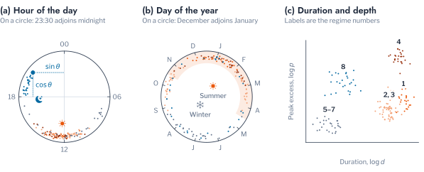
The composite score selected eight regimes, with a separation score of 0.701 and a trust factor of 0.949, against a composite of 0.529 for the next candidate, three regimes. Table 4.3 describes them in order of total duration. Four regimes accounted for 89.0% of the 745,969.5 hours of violation. Regime 1 is the summer midday over-voltage, with events centred at noon that lasted 5.28 hours on average, all in the summer half-year and most frequent in January. Regimes 2 and 3 are the same phenomenon in the shoulder seasons, with modal months of October and March and mean durations of 4.0 hours. Regime 4 is the reverse-flow overload, comprising 22,237 events, all of them overloads and almost all in summer, which lasted 5.11 hours with a median excess of 0.37 of the rating and occurred at a mean PV penetration of 0.75, the highest of any regime. Regimes 5 to 7 contain brief and shallow over-voltages of about one hour, on winter middays and at the morning and afternoon edges of summer days. Regime 8 is the only evening regime, with events centred at 19:15 that lasted 1.31 hours, divided between under-voltage (59%) and overload (40%), at a mean EV penetration of 0.66.
Figure 4.10 places a sample of the events of each regime on these features. The midday regimes of PV occupy the hours around noon at durations of several hours and are separated by season, the reverse-flow overload of Regime 4 lies above the over-voltages in depth, and Regime 8 is the only regime centred in the evening. The regimes therefore cut across the limit types in a way that matters for operation. Overload appears in two regimes with opposite causes, reverse flow at noon in Regime 4 and charging in the evening in Regime 8, which call for opposite remedies, and midday over-voltage divides by season into regimes whose durations differ by more than an hour.
Figure 4.11 shows how the regimes emerged as penetration grew. Without DER the network recorded only Regime 8, for 65.5 hours over the year. PV at 20% brought the three over-voltage regimes at once, with 3,666.5 hours of Regime 1 and 1,557.5 to 1,887.5 hours of Regimes 2 and 3, together with the short Regimes 5 to 7. Each regime grew with penetration, but at a different rate: the short Regimes 6 and 7 saturated near 1,200 hours, whereas Regime 1 reached 19,370.0 hours at 80%. Regime 4 was absent below 40% PV, appeared with 85.0 hours at 40% and grew to 5,349.0 hours at 60% and 19,832.0 hours at 80%, when it overtook Regime 1 as the largest regime. EV adoption, in contrast, enlarged a single regime, Regime 8, from 229.0 hours at 20% to 1,921.0 hours at 80%. Since the network records no over-voltage without PV, the few hours that EV adoption placed in other regimes are under-voltages and overloads whose timing and depth assign them there: 38.5 hours of the brief Regime 6 at 80% EV, and at most 3.0 hours in each of Regimes 1, 3, 4 and 5. The dominant regime thus changes with penetration, from midday over-voltage at low PV penetration to reverse-flow overload at 80%, a transition that the four limit types record only as a growth in total hours.
Demand at the Time of Violation
The regimes describe when and how the network fails, but not which customers are drawing power when it does. The correlations of Network Response to DER Penetration average over the whole year, whereas a violation is decided by the demand present during the few hours in which it occurs. The event record and the household time series together allow this demand to be measured directly. For every violation in the three extreme scenarios, the demand of each customer on the affected transformer during the event is compared with the same household’s mean demand at the same half-hour of the day over the year (Table 4.4). For the set \(\mathcal{P}_A\) of customer and half-hour pairs \((i, t)\) of archetype \(A\) in violation, the ratio to usual demand is
\[ \rho_A = \frac{\sum_{(i, t) \in \mathcal{P}_A} x_{i,t}}{\sum_{(i, t) \in \mathcal{P}_A} \bar{x}_{i, \tau(t)}}, \tag{4.3}\]
where \(\bar{x}_{i, \tau}\) is the mean demand of household \(i\) at half-hour \(\tau\) of the day over the year and \(\tau(t)\) the half-hour of the day of step \(t\).
The two regimes differed in how demand participated. During PV-driven over-voltage, households drew close to their usual demand for the hour, at ratios \(\rho_A\) of 0.936 to 0.968 for the three archetypes, which confirms that these violations are driven by generation rather than by unusual consumption. Archetypes 2 and 3 drew 0.620 and 0.537 kW per customer during these events against 0.333 kW for Archetype 1, so that their higher daytime base absorbed more of the local export. During EV-driven violations, households of every archetype drew 1.62 to 1.92 times their usual demand at the same hour, because these violations occur on the evenings of highest household demand, when the charging load is added to an already elevated base.
Across households, however, the archetype explained little of the demand present at these moments: 15.5% of its variance during over-voltage, 9.4% during under-voltage and 8.5% during overload. The household’s annual mean demand, by contrast, correlated with it at 0.928, 0.806 and 0.744 respectively. The demand that coincides with a violation is therefore determined chiefly by how much a household consumes, and the timing that distinguishes the archetypes accounts for a small part of it, larger during the midday regime than during the evening one.
Attribution of Risk to Archetypes
Both the transformer-level correlations and the event-time demand relate archetypes to risk through aggregates. This section attributes risk to individual customers and measures how much of its variation the archetype captures. Two one-day scenarios are solved on HPK11 with every customer equipped, so that differences between customers arise only from their demand and their location. In the first, every customer has a 5 kVA array, on a day at the end of December. In the second, every customer has a 7.36 kW charger operating from 18:00 to 21:00 on a day in mid-January, the day of highest aggregate evening demand, whose network peak falls at 19:00. The voltage scenario is deliberately severe, with worst voltages from 1.098 to 1.235 pu and 99.9% of customers above 1.10 pu at some half-hour, while the contribution to the evening peak ranged from 2.54 to 15.99 kW.
The three archetypes were indistinguishable in voltage and close in thermal outcome (Table 4.5). Their mean worst voltage differed by 0.001 pu and their mean time above the limit by 0.13 half-hours. Their mean contribution to the peak differed by 0.99 kW, from 6.60 kW for Archetype 1 to 7.59 kW for Archetype 2, against a range across customers of 13.45 kW, and their distributions over households overlap almost entirely (Figure 4.12).
To locate the variation that the archetypes miss, Figure 4.13 decomposes the variance of each outcome across the 5,274 customers into the shares explained by the customer’s archetype, by the tercile of its household’s annual mean demand, by both together, by its household and by its LV transformer. For an outcome \(y_i\) of customer \(i\) and a grouping \(g\) of the customers into groups \(G\) of \(n_G\) customers with mean \(\bar y_G\), the share explained is the correlation ratio, or eta squared [12],
\[ \eta^2 = \frac{\sum_{G} n_G \, (\bar y_G - \bar y)^2}{\sum_{i} (y_i - \bar y)^2}, \tag{4.4}\]
the share of the variance of \(y\) that lies between the groups. The household share bounds what any grouping of households can explain, since a segment can only average households together.
Location dominated voltage. The transformer explained 69.3% of the variance of the worst voltage and 52.1% of the time above the limit, against 6.4% and 6.7% for the household and nothing to three decimal places for the archetype. The thermal outcome showed the reverse pattern, with the household explaining 69.6% of the contribution to the peak and the transformer 17.6%. The archetypes captured little of this household share, 5.3% at the chosen \(K = 3\), 0.2% at \(K = 2\) and 9.5% at \(K = 11\), whereas a single attribute of magnitude, the tercile of annual demand, explained 12.7% on its own and 16.5% together with the archetype. Figure 4.14 illustrates the two mechanisms: the voltage a customer experiences depends on where it connects, whereas the loading of a transformer is the sum of what its customers draw.
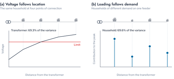
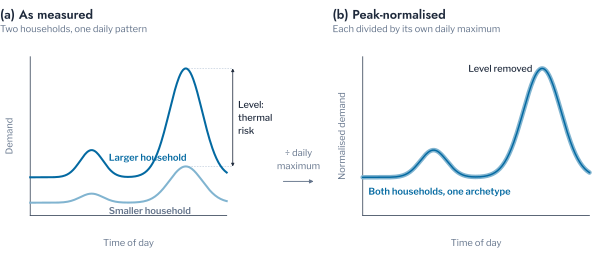
Table 4.6 identifies the magnitude that matters. A household’s demand at the half-hour of the network peak correlated with its contribution to that peak at 0.982, and its mean demand over the year at 0.543, whereas no demand feature correlated with the worst voltage beyond 0.07 in absolute value, because with every customer exporting, the voltage a customer experiences is set by its point of connection. The pipeline divides each household’s readings by its own daily maximum precisely in order to remove magnitude, so that the archetypes describe when a household consumes rather than how much. The thermal risk therefore resides in what this normalisation discards (Figure 4.15).
Conclusion
This chapter examined the network risk that rooftop PV and EV charging impose on HPK11 and asked whether the archetypes of Chapter 3 carry it. The response of the network was governed by technology, location and magnitude rather than by the archetypes. Over-voltage depended almost entirely on PV and limited the hosting capacity of most transformers already at 20%, reverse power flow dominated the thermal exposure, and the exposure of each transformer followed its number of customers and its loading ratio rather than its archetype mix. Clustering the 221,070 violation events produced eight regimes, which separated reverse-flow overload at noon from charging overload in the evening and showed reverse-flow overload, absent below 40% PV penetration, becoming the largest regime at 80%.
At the level of the customer, location determined voltage risk and the level of demand determined thermal risk. The transformer explained 69.3% of the variance of the worst voltage, the household 69.6% of the contribution to the evening peak, and the archetypes none of the first and 5.3% of the second, because peak normalisation removes the level of demand on which thermal risk depends. Chapter 5 therefore turns to segmentations that retain the level of demand, and to the uses of clustering in network studies that depend on it.
Key findings
Network risk on HPK11 followed technology, location and the level of demand, not the shape of demand. Over-voltage limited the hosting capacity for PV before loading did, and the exposure of a transformer followed its number of customers and its loading ratio. Clustering the violation events into regimes separated reverse-flow overload at noon from charging overload in the evening and revealed a change in the dominant regime as PV penetration grew. The transformer explained most of the variance of voltage risk and the household most of the thermal risk, whereas the shape archetypes explained 5.3% of the thermal risk and none of the voltage risk.
Exercises
- In the
regimescell of the companion notebook, add the peak loading of the transformer during each event as a further feature of Equation 4.2. Does Regime 4, the reverse-flow overload, separate further from the over-voltage regimes? - Replace the terciles of annual demand in the
variancecell with quintiles. How close does a quintile of annual demand come to the household share of the contribution to the peak? - Compute, for each transformer, the share of its violation hours in each regime at 80% PV. Do transformers with the same dominant regime share a loading ratio?
References
Karunarathne, Pereira Guzman and Ochoa, MV-LV-Networks: four real Australian MV/LV distribution networks with real demand profiles, https://github.com/Team-Nando/MV-LV-Networks.↩︎