Foundations of Load-Profile Clustering
The binding constraint of the energy transition at the distribution level is the low-voltage network, which was designed decades before bidirectional power flows were anticipated. Rooftop solar, residential storage and Electric Vehicle (EV) chargers are connected property by property, and a Distribution System Operator (DSO) frequently learns of their combined effect only when a feeder trips or a transformer overheats. Monitoring each customer individually is feasible for a feeder of a few hundred customers and infeasible at the scale of a national network. Clustering, which Wang, Chen, Hong and Kang identify as one of the three pillars of smart-meter analytics alongside forecasting and load management [1], addresses this problem of scale: it reduces a large population of individual customers to a small number of recurring consumption patterns on which planning, tariff design and demand response can operate.
The reduction, however, has no unique answer. Each household of a metered population follows its own daily pattern, and the average of the population describes few of them well. Jain’s review of fifty years of clustering research identifies the underlying difficulty: the choice of objective function is itself a modelling decision rather than a property of the data [2]. Before a single customer is clustered, therefore, four questions have to be settled. The first is what formal criterion makes two customers, or two feeders, members of the same group. The second is whether a load curve needs a specialised notion of distance and representation, or whether a standard one suffices. The third is how a grouping can be shown to be valid when no labels exist to check it against. The fourth is how physical knowledge, such as the feeder to which a customer is connected, can shape the clustering itself rather than only annotate its result.
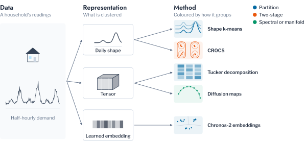
This chapter prepares the ground for answering them. It introduces the notation used throughout Part 5, reviews the objective families, representations, validity indices and stability measures on which later chapters rely, and illustrates the behaviour of each on a synthetic population whose structure is known in advance. Chapter 2 answers the first three questions on metered data from three utilities, Chapters 3 to 5 apply the resulting pipeline to customer archetypes, network risk and network studies, and Chapter 7, in preparation, returns to the fourth once customers are clustered on a physical feeder. Figure 1.1 places the methods of the part relative to one another.
Load-Profile Clustering in the Literature
The questions above are not new, and the energy literature has approached them in two broad phases. The first phase compared clustering methods on load profiles. Chicco’s overview was the first to set methods for load-pattern grouping side by side rather than to introduce a single method in isolation [3]. McLoughlin, Duffy and Conlon, Kwac, Flora and Rajagopal, and Haben, Singleton and Grindrod then established that clusters built on the shape of a load curve correspond to observable household behaviour rather than to statistical artefacts [4], [5], [6]. Rajabi et al. extended this line towards systematic benchmarking of clustering techniques for load patterns [7], and Michalakopoulos et al. compared k-means, k-medoids, hierarchical clustering and DBSCAN on the London population that Chapter 2 also uses [8].
The second phase replaced hand-engineered features with learned representations. Deep Embedded Clustering [9] and its improved variant [10] have been surveyed by Ezugwu et al. [11], by Ren et al. [12] and, for time series specifically, by Alqahtani et al. [13]. Applications range from linking clustered peak-demand profiles to occupant activity [14] to an autoencoder-based load-profiling framework [15]. The CROCS framework of Yerbury et al. is the closest precedent to this part: it summarises each consumer by a set of representative daily behaviours and then clusters consumers by the similarity of those sets [16].
Across both phases, two gaps recur. Findings are rarely tested on a second, independently collected population, and few studies compare more than a small number of clustering paradigms under a common protocol. This part addresses both by applying every comparison to three utilities. Doing so requires a common vocabulary, which the next section introduces.
Notation and an Illustrative Population
Consider a population of \(N\) meters, each recording \(T\) readings per day over \(D\) days. The mean daily profile of meter \(i\) is \(\mathbf{x}_i \in \mathbb{R}^{T}\), and its peak-normalised shape is
\[ \mathbf{s}_i = \frac{\mathbf{x}_i}{\max_{t} x_{i,t}}, \]
which keeps the timing of consumption and discards its magnitude. A clustering assigns each meter a label \(\lambda(i) \in \{1, \dots, K\}\) and so defines a partition \(\mathcal{C} = \{C_1, \dots, C_K\}\) with cluster sizes \(n_k = |C_k|\). Table 1.1 collects the notation used in the remainder of the part.
| Symbol | Description |
|---|---|
| \(N\), \(T\), \(D\) | Number of meters, readings per day and days |
| \(\mathbf{x}_i \in \mathbb{R}^{T}\) | Mean daily profile of meter \(i\) |
| \(\mathbf{s}_i \in [0, 1]^{T}\) | Peak-normalised shape of meter \(i\) |
| \(\mathcal{X} \in \mathbb{R}^{N \times D \times T}\) | Meter-by-day-by-reading tensor |
| \(K\) | Number of clusters |
| \(\mathcal{C} = \{C_1, \dots, C_K\}\) | Partition; \(n_k = \lvert C_k \rvert\) |
| \(\lambda(i)\) | Cluster label of meter \(i\) |
| \(\mathbf{c}_k\) | Centroid of cluster \(k\) |
| \(d(\cdot, \cdot)\) | Distance between two profiles |
| \(p_k = n_k / N\) | Population share of cluster \(k\) |
| \(\alpha\), \(\hat q\), \(\Gamma(i)\) | Miscoverage level, conformal threshold and conformal set of meter \(i\) (Chapter 3) |
| \(\eta^2\) | Share of the variance of an outcome explained by a grouping (Chapter 4) |
| \(r_{i,t}\), \(\tilde r_{i,t}\) | Representative and scaled representative reading of household \(i\) (Chapter 5) |
| \(x_t\), \(L\), \(e_t\) | Network series at step \(t\), its limit and the excess beyond the limit (Chapter 4) |
| \(d\), \(I\), \(\Delta\) | Duration and integral of a violation event, and the time step (Chapter 4) |
The concepts of this chapter are easier to judge against a population whose structure is known, so each is illustrated on a synthetic one. One hundred and twenty households are drawn from four daily archetypes with evening, morning, daytime and night peaks (Figure 3.2). Each household has its own magnitude, a daily time shift and multiplicative noise, and household peak demand ranges from 0.05 kW to 40.05 kW. The range deliberately exceeds that of any real population, so that magnitude dominates every distance computed on raw demand and the contrast between magnitude and shape examined below is unambiguous. To mimic the imperfections of metered data, four meters without a daily routine and one vacant property reporting a constant 0.02 kW are added; the vacant property is removed during preparation, which leaves 124 meters. Because the archetypes are known, every method can be scored by the adjusted Rand index (ARI) of its partition against the planted labels, a measure defined formally later in the chapter.
Four Definitions of a Cluster
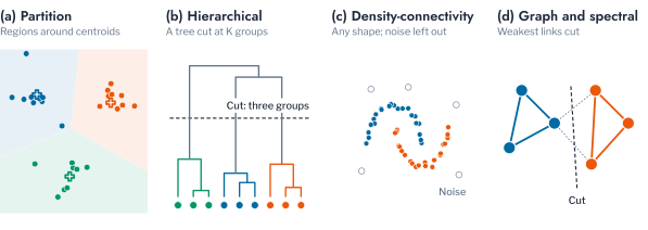
The first question, what makes two customers members of the same group, has no single answer. Four objective families account for the clustering methods used in this part, and each defines a cluster through a different criterion, so the same population can yield different partitions under each [2].
Partition-based objectives place \(K\) centroids so as to minimise the distance of each point to its nearest centroid. For k-means the objective is the within-cluster sum of squares,
\[ J(\mathcal{C}) = \sum_{k=1}^{K} \sum_{i \in C_k} \lVert \mathbf{s}_i - \mathbf{c}_k \rVert^2, \qquad \mathbf{c}_k = \frac{1}{n_k} \sum_{i \in C_k} \mathbf{s}_i, \tag{1.1}\]
which alternating assignment and update steps reduce to a local minimum. These objectives follow MacQueen’s k-means formulation and Lloyd’s algorithm, with the seeding of Arthur and Vassilvitskii reducing sensitivity to initialisation [17], [18]. Hierarchical objectives instead build a tree by repeatedly merging the two closest groups under a linkage rule. Single linkage measures the closest cross-group pair, \(d_{SL}(G,H) = \min_{i \in G, i' \in H} d_{i,i'}\), complete linkage the farthest pair, \(d_{CL}(G,H) = \max_{i \in G, i' \in H} d_{i,i'}\), and average linkage the mean over all cross-group pairs, \(d_{avg}(G,H) = \frac{1}{n_G n_H} \sum_{i \in G} \sum_{i' \in H} d_{i,i'}\); Ward’s minimum-variance criterion belongs to the same family [19].
Density-connectivity objectives dispense with a fixed number of clusters altogether and group points into chains of dense neighbourhoods. In DBSCAN, a point is a core point when it has a minimum number of neighbours within a given radius, a border point when it neighbours a core point without satisfying that condition itself, and noise otherwise [20]. Graph-based and spectral objectives, finally, treat the population as a similarity graph and partition it along its weakest connections. Ng, Jordan and Weiss minimise the normalised cut
\[ \text{Ncut}(S_1, \dots, S_K) = \frac{1}{2} \sum_{k=1}^{K} \frac{\text{cut}(S_k, \bar{S}_k)}{\text{vol}(S_k)}, \tag{1.2}\]
where \(\text{cut}(S_k, \bar{S}_k) = \sum_{i \in S_k, j \notin S_k} w_{ij}\) is the similarity crossing the cut and \(\text{vol}(S_k) = \sum_{i \in S_k} d_i\) the total degree within \(S_k\); the relaxed problem is solved with the eigenvectors of the graph Laplacian \(L = D - W\) [21]. Figure 1.3 contrasts the four.
The families also differ in computational cost, which becomes a selection criterion at utility scale. Partition-based methods scale as \(O(NKdI)\) for \(d\) dimensions and \(I\) iterations, which makes them the practical default for large populations. Hierarchical methods require \(O(N^2)\) memory and \(O(N^3)\) time in the naive implementation, reducible to \(O(N^2 \log N)\) with a priority queue. DBSCAN costs \(O(N \log N)\) with a spatial index and \(O(N^2)\) without one, and spectral methods are typically the most expensive, at \(O(N^3)\) for the eigendecomposition of the Laplacian.
On the synthetic population, these differences in definition become differences in outcome (Table 1.2). Partition, Ward, density, spectral and mixture methods all recovered the four archetypes exactly, with an ARI of 1.000, whereas average linkage reached 0.709 because a single irregular meter sufficed to merge two groups under the average-distance rule. The more instructive difference concerns the four irregular meters. DBSCAN and HDBSCAN labelled all four as noise, while every method that must assign each point to some cluster absorbed them into an archetype to which they do not belong. Whether the population contains points that belong to no group is therefore part of the choice of objective, not a detail to be handled afterwards.
Distance and Representation
Every objective family operates on distances, which raises the second question: distances between what, and measured how? A load curve differs from generic tabular data in two respects that matter here. Its magnitude varies by orders of magnitude across households, and its timing can drift from one household to another. This section considers each in turn, then turns to richer representations and to the dimensionality they introduce.
Shape Before Magnitude
Two households can differ in absolute demand by more than an order of magnitude and still follow the same daily rhythm. A clustering of the mean daily load \(\mathbf{x}_i\) therefore separates households by size, whereas a clustering of the shape \(\mathbf{s}_i\) separates them by behaviour. The synthetic population makes the contrast concrete (Table 1.3). k-means on the mean daily load attained an ARI of 0.001 against the archetypes, and its clusters were bands of household size with median peaks of 0.88, 5.35, 18.06 and 40.05 kW. The same algorithm on peak-normalised shapes attained an ARI of 1.000, with the median peak of every cluster between 0.84 and 1.45 kW. Figure 1.4 shows the cluster means behind these numbers. For this reason, every method in this part clusters on shape.
Elastic Alignment
Normalising magnitude still leaves timing. Two households with the same routine may be offset by a fraction of an hour, which a point-by-point Euclidean comparison registers as a mismatch. Dynamic time warping (Dynamic Time Warping (DTW)), introduced by Sakoe and Chiba for spoken-word recognition, addresses this by computing the cost of the best monotonic alignment between two series by dynamic programming [22]. For \(\mathbf{x} = (x_1, \dots, x_n)\) and \(\mathbf{y} = (y_1, \dots, y_m)\),
\[ D(i, j) = d(x_i, y_j) + \min\{D(i-1, j),\ D(i, j-1),\ D(i-1, j-1)\}, \tag{1.3}\]
with \(D(0, 0) = 0\) and all other boundary cells set to infinity; the DTW distance is \(D(n, m)\). Aghabozorgi, Shirkhorshidi and Wah regard the choice of representation and distance as an open question of time-series clustering rather than one settled by general clustering theory [23], and Figure 1.5 illustrates why warping is attractive in principle.
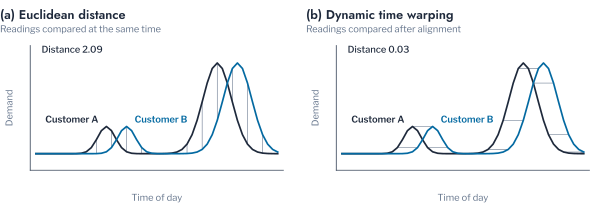
Whether warping improves a clustering depends on whether timing carries information. Table 1.4 shifts each household’s profile by a random number of half-hours and clusters the result under both distances. For shifts of up to 1.5 hours, Euclidean distance recovered the archetypes exactly while unconstrained DTW reached an ARI of 0.62, and at 2.5 hours the values were 0.97 and 0.52. Only when shifts reached 4 hours, by which point Euclidean distance had degraded to 0.34, did DTW perform better, at 0.43. The reason is that the archetypes are defined by the time of their peak, and unconstrained warping aligns peaks that occur at different times of day. Euclidean distance on time-aligned, peak-normalised profiles is therefore the default adopted in this part for regularly sampled Advanced Metering Infrastructure (AMI) data. A Sakoe-Chiba band, which limits how far the alignment may stretch, is not evaluated here.
Tensor and Manifold Representations
A mean daily profile summarises a season in a single curve. Two further representations retain more of its structure. The readings of a population over a season form a three-way array \(\mathcal{X} \in \mathbb{R}^{N \times D \times T}\) indexed by meter, day and reading, and Tucker’s decomposition factorises such a tensor into a core tensor and one factor matrix per mode, \(\mathcal{X} \approx \mathcal{G} \times_1 \mathbf{A} \times_2 \mathbf{B} \times_3 \mathbf{C}\), generalising the matrix factorisation that underlies principal component analysis [24]. The rows of the meter factor \(\mathbf{A}\) then represent each meter. Diffusion maps take a nonlinear route to a similar end: a kernel similarity defines a Markov transition matrix \(P = D^{-1} W\), and the embedding \(\Psi_t(i) = (\lambda_1^t \psi_1(i), \lambda_2^t \psi_2(i), \dots)\) scales each leading eigenvector by its eigenvalue raised to the diffusion time \(t\) [25]. Both recover the synthetic archetypes exactly (Table 1.3); whether they add information on metered data is the subject of Chapter 6, in preparation.
Any of these representations is only as reliable as the data from which it is computed, and metered data rarely arrives ready for clustering.
Remark: preparation of metered data
Aghabozorgi, Shirkhorshidi and Wah treat preparation as a stage of its own, separate from the choice of distance [23]. A gap caused by a missed read is interpolated or the affected period excluded; filling it with zeros introduces an artificial trough. Every meter is placed on a common, regular time grid, and meters with insufficient coverage are excluded. On the synthetic population, a three-hour gap is interpolated from the adjacent readings, and a meter missing three quarters of its week is removed, leaving 123 of 124 meters with at least 90% coverage. The aggregation window is itself a modelling decision: a short window confuses a single atypical day with a household’s pattern, while a long window can average away the behavioural change that later chapters set out to detect.
Dimensionality
Richer representations bring more dimensions, and more dimensions are not necessarily more information.
Pitfall: adding features
As dimensionality grows towards the size of the population, pairwise distances concentrate, and a clustering algorithm can report partitions induced by noise rather than by structure. Ezugwu et al. and Ren et al. both list the curse of dimensionality among the open problems of clustering [11], [12].
Dimensionality reduction addresses this problem but raises another: how many components to retain. A fixed rule, such as keeping the components that explain 90% of the variance, is common but arbitrary. Zhu and Ghodsi’s profile-likelihood method instead locates a change point in the ordered eigenvalues \(\lambda_1 \geq \dots \geq \lambda_p\) without any threshold [26]. The first \(q\) eigenvalues and the remaining \(p - q\) are modelled as two Gaussian groups with a pooled variance, and \(q\) is chosen to maximise
\[ \ell(q) = \sum_{i=1}^{q} \log \mathcal{N}(\lambda_i \mid \mu_1, \sigma^2) + \sum_{i=q+1}^{p} \log \mathcal{N}(\lambda_i \mid \mu_2, \sigma^2), \tag{1.4}\]
where pooling \(\sigma^2\) across both groups prevents the likelihood from diverging as one group’s variance shrinks to zero. On the synthetic population the two rules already disagreed (Figure 1.6): the 90% variance rule retained four principal components, while profile likelihood retained two, which together explain 72.8% of the variance. Chapter 2 compares the two rules on metered data, where the disagreement is larger.
The synthetic population was free of anomalies by construction apart from the meters added to it. Metered populations are not, and the last consideration of representation concerns what is clustered at all.
Pitfall: populations that are not homogeneous
A population passed to a clustering algorithm is not necessarily a single population. A vacant property reports a near-constant reading that resembles a distinct archetype, and a faulty meter reports stuck or clipped values that resemble an extreme behaviour; neither is behaviour to be clustered. Residential and commercial customers, or customers in different climates, are likewise distinct populations for shape-based clustering, irrespective of a shared billing category. In the synthetic population, the vacant property is removed before clustering because its readings do not vary.
Background Knowledge as a Constraint
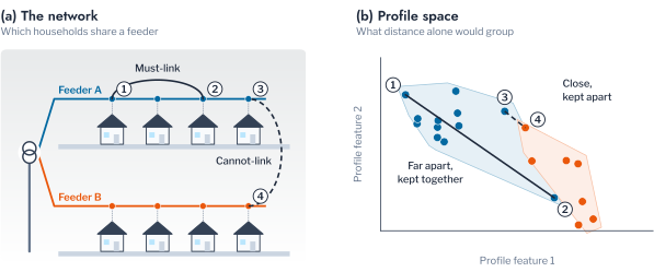
The fourth question asks whether knowledge from outside the meter data can shape the clustering itself. Distance alone cannot know that two customers share a feeder, yet a utility often does. Wagstaff, Cardie, Rogers and Schrödl’s COP-KMeans makes such knowledge part of the assignment step of k-means through two types of side information: a must-link constraint requires two points to share a cluster, and a cannot-link constraint forbids it. Assignments that violate either constraint are rejected rather than penalised [27], as Figure 1.7 illustrates. Chapter 7, in preparation, uses this vocabulary to cluster customers on a common physical feeder under the constraints that the network topology imposes; it is not evaluated on the synthetic population.
Judging a Partition Without Labels
With a definition, a distance and a representation in place, a clustering produces a partition. The third question is whether that partition is valid, and in the absence of labels the first line of evidence is internal: indices that combine within-cluster compactness with between-cluster separation. The silhouette coefficient of Rousseeuw compares how well each point fits its own cluster with how well it would fit the nearest other cluster [28],
\[ s(i) = \frac{b(i) - a(i)}{\max\{a(i), b(i)\}}, \tag{1.5}\]
where \(a(i)\) is the mean distance from point \(i\) to the other members of its cluster and \(b(i)\) the mean distance to the members of the nearest other cluster. The Davies-Bouldin index takes the perspective of the clusters rather than the points, comparing each cluster with its least separated neighbour [29],
\[ DB = \frac{1}{K} \sum_{i=1}^{K} \max_{j \neq i} \left( \frac{\sigma_i + \sigma_j}{d(\mathbf{c}_i, \mathbf{c}_j)} \right), \tag{1.6}\]
where \(\sigma_i\) is the mean distance of the members of cluster \(i\) to its centroid \(\mathbf{c}_i\), so that lower values indicate better separation. The Caliński-Harabasz index expresses the same idea as a variance ratio [30],
\[ CH = \frac{SS_B / (K - 1)}{SS_W / (N - K)}, \tag{1.7}\]
where \(SS_B\) is the size-weighted squared distance of the centroids to the overall mean and \(SS_W\) the squared distance of every point to its centroid; higher values indicate better separation.
Because the three indices are built from the same two quantities, they share a limitation: none contains a term for population share, so a small group of distant points satisfies every one of them, whatever its size. The balance of a partition supplies the missing term through the normalised entropy of the cluster sizes [31],
\[ H(\mathbf{p}) = -\frac{1}{\log K} \sum_{k=1}^{K} p_k \log p_k, \tag{1.8}\]
which equals one when all clusters have the same size and approaches zero when one cluster holds almost the entire population. Table 1.5 and Figure 1.8 show the limitation on 62 points, 60 drawn from one Gaussian cloud and two placed far from it. Treating the two outliers as a cluster yielded a silhouette of 0.911, a Caliński-Harabasz index of 379.4 and a Davies-Bouldin index of 0.076, against 0.195, 9.5 and 1.253 for a split of the main cloud, so all three indices preferred the outlier partition. Balance alone distinguished the two, at 0.206 for the outlier partition and 0.997 for the split. Balance is a diagnostic rather than a proof, however, since a genuine minority archetype lowers it too.
Choosing the Number of Clusters
Internal indices are most often used to choose \(K\), and the limitation just described carries over directly. The number of clusters is commonly read from the elbow of the inertia curve, but inertia decreases monotonically with \(K\), since every additional cluster reduces within-cluster distances, and its elbow is frequently ambiguous. Figure 3.1 therefore shows how each validity index ranks \(K\) from 2 to 9 on the synthetic population, and Table 8.2 lists the number of clusters each selection rule recommends. Davies-Bouldin recovered the planted four clusters, but the silhouette, the Caliński-Harabasz index, the majority of the three and the weighted Borda rank all recommended five, and the inertia elbow recommended eight. At \(K = 5\) the clusters contained 30, 30, 30, 30 and 4 meters, and the cluster of four consisted exactly of the irregular meters: a compact, well-separated group of the kind that Table 1.5 showed the separation indices reward. No single index is sufficient, which is why later chapters consult several of them together with the resampling evidence introduced next.
Stability and Agreement
Internal indices judge a single partition. A complementary line of evidence asks whether the partition reappears when the algorithm or the data are perturbed, on the reasoning that structure present in the population should survive both.
Perturbing the algorithm is the simplest case. The cluster-based similarity partitioning approach of Strehl and Ghosh runs the algorithm \(r\) times on the same objects [32] and records, in a co-association matrix
\[ S_{ij} = \frac{1}{r} \sum_{m=1}^{r} \mathbb{1}\left[\lambda_m(i) = \lambda_m(j)\right], \tag{1.9}\]
the share of runs that place objects \(i\) and \(j\) in the same cluster. Blakely and Reno applied the same construction to the identification of the phase to which each customer is connected [33]. Over twenty k-means runs on the synthetic population, the mean co-association was 1.00 within archetypes and 0.02 across them, and the consensus partition recovered the archetypes exactly.
Perturbing the data asks more. Tibshirani and Walther’s prediction strength treats clustering as an implicit classification problem [34]: the data are split into halves \(A\) and \(B\), each half is clustered into \(K\) groups, and the centroids of \(A\) are used to predict the membership of \(B\). For each cluster \(C\) of \(B\),
\[ \text{ps}(C) = \frac{1}{n_C (n_C - 1)} \sum_{\substack{i, i' \in C \\ i \neq i'}} \mathbb{1}\left[\text{pred}(i) = \text{pred}(i')\right], \tag{1.10}\]
and the prediction strength of \(K\) is the minimum of \(\text{ps}(C)\) over the clusters of \(B\). Tibshirani and Walther recommend the largest \(K\) with prediction strength above 0.8 to 0.9. Where prediction strength judges \(K\) as a whole, Hennig’s cluster-wise stability judges each cluster separately [35]. The data are resampled with replacement and clustered, and each original cluster \(C\) is matched to its most similar cluster \(C'_b\) in resample \(b\),
\[ \text{stability}(C) = \frac{1}{B} \sum_{b=1}^{B} \max_{C'_b} \frac{|C \cap C'_b|}{|C \cup C'_b|}. \tag{1.11}\]
Hennig reads stability below 0.5 as dissolved, 0.6 to 0.75 as patterned but not stable, and above 0.75 as stable. Figure 1.10 contrasts the two mechanisms.
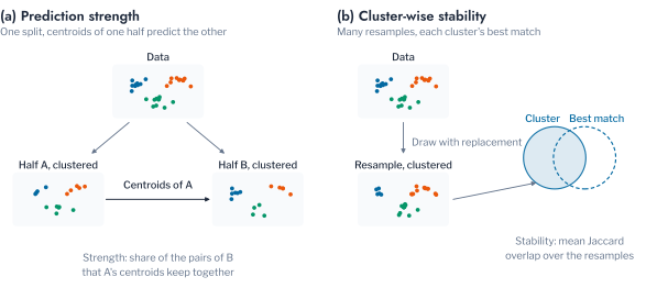
Applied to the synthetic population, both measures supported the planted structure but did not single it out (Table 1.7). At \(K = 4\), prediction strength was 0.822 and the least stable cluster had a stability of 0.953, with the four archetypes between 0.949 and 0.986. At \(K = 5\), the values rose to 0.900 and 1.000, because the cluster of irregular meters was as reproducible as the archetypes. At \(K = 7\) they fell to 0.594 and 0.392. Resampling thus establishes that a grouping is reproducible, which is necessary but does not establish that the grouping is meaningful.
A further subtlety affects any comparison across \(K\): both measures change with \(K\) even in data that contain no clusters at all. Comparing each measure with its value on structureless reference data of the same size and range removes this dependence. On uniform reference data, prediction strength fell from 0.507 at \(K = 2\) to 0.131 at \(K = 6\) (Table 1.8), so a raw comparison would favour small \(K\). The excess of the observed value over the reference was small at \(K = 2\), at 0.074, and between 0.48 and 0.58 for \(K\) from 3 to 6. Averaged over the three resampling checks, it was largest at \(K = 5\), at 0.725 (Figure 1.11). Chapter 2 relies on this calibration when it compares candidate values of \(K\) on metered data.
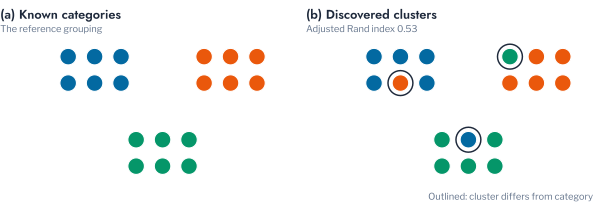
Every comparison in this section, and every score against the planted archetypes in this chapter, rests on a measure of agreement between two partitions of the same objects. The adjusted Rand index of Hubert and Arabie counts the pairs of objects on whose co-membership two partitions agree, subtracts the agreement expected by chance, and rescales so that identical partitions score one and chance agreement scores zero [36]:
\[ \text{ARI} = \frac{\sum_{ij} \binom{n_{ij}}{2} - \left[ \sum_i \binom{a_i}{2} \sum_j \binom{b_j}{2} \right] / \binom{n}{2}}{\frac{1}{2} \left[ \sum_i \binom{a_i}{2} + \sum_j \binom{b_j}{2} \right] - \left[ \sum_i \binom{a_i}{2} \sum_j \binom{b_j}{2} \right] / \binom{n}{2}}, \tag{1.12}\]
where \(n_{ij}\) is the number of objects in group \(i\) of one partition and group \(j\) of the other, and \(a_i\) and \(b_j\) are the group sizes. The normalised mutual information of Strehl and Ghosh measures the same agreement through information rather than pairs, as the reduction in uncertainty about one partition given the other [32],
\[ \text{NMI}(U, V) = \frac{I(U, V)}{\frac{1}{2} \left[ H(U) + H(V) \right]}, \tag{1.13}\]
where \(I(U, V)\) is the mutual information of the two partitions and \(H(\cdot)\) the Shannon entropy. Neither index rewards a partition for having the same number of groups as another; both reward only the grouping of the same objects, as Figure 1.12 illustrates.
Validation Against a Controlled Change
Internal indices, balance, ensemble agreement and resampling stability all describe how well a partition is structured, yet none of them confirms that the partition corresponds to real behaviour. A controlled change with a known outcome provides that confirmation. In the synthetic population, fifteen households of the morning archetype adopt overnight EV charging between 21:00 and 01:00. If the clustering responds to behaviour, these households should leave the morning archetype and form a cluster of their own. For the set \(\mathcal{A}\) of changed households and the cluster \(C\) that holds most of them, the recovery is measured by
\[ \text{recall} = \frac{\lvert \mathcal{A} \cap C \rvert}{\lvert \mathcal{A} \rvert}, \qquad \text{purity} = \frac{\lvert \mathcal{A} \cap C \rvert}{\lvert C \rvert}, \qquad \text{Jaccard} = \frac{\lvert \mathcal{A} \cap C \rvert}{\lvert \mathcal{A} \cup C \rvert}. \tag{1.14}\] At \(K = 5\) they did: all fifteen fell in a single cluster that contained no other household, with a recall, purity and Jaccard overlap of 1.00 (Table 1.9). Chapter 3 applies the same test to metered households, where the outcome is less definite.
Conclusion
This chapter set out the questions that Part 5 addresses and the instruments it uses to answer them. On a synthetic population with four planted archetypes, four irregular meters and one vacant property, the illustrations showed that the choice of objective already determines how outliers are treated: every family except average linkage recovered the archetypes exactly, but only the density-based methods set the irregular meters aside as noise. They showed that the representation matters more than the algorithm, since k-means reached an ARI of 0.001 on mean daily load and 1.000 on peak-normalised shape, and that unconstrained dynamic time warping performed worse than Euclidean distance for time shifts of up to 2.5 hours, because the archetypes are defined by the timing of their peak. The two rules for retaining components disagreed even on data free of anomalies, at four and two components.
The illustrations also exposed the main weakness of internal evaluation. Three separation indices preferred a partition that isolates two outliers, and four of six selection rules chose five clusters on the synthetic population by isolating the irregular meters. Resampling confirmed that this cluster was reproducible without showing whether it was meaningful, and only a controlled behavioural change, recovered with a recall and purity of 1.00, tied a cluster to behaviour. Separation indices therefore have to be read together with balance, calibrated resampling evidence and, where possible, an external check.
These conclusions rest on a population that is free of anomalies by construction, and two of the methods introduced here, constrained clustering and a warping window for dynamic time warping, were not evaluated. Chapter 2 applies the same instruments to metered data from three utilities, where none of the structure is known in advance, and uses them to settle the first three questions of this chapter.
Key findings
The choice of objective determined how irregular meters were treated: only the density methods set them aside as noise. Clustering on peak-normalised shape recovered the planted archetypes exactly, where clustering on magnitude recovered none of them, and Euclidean distance outperformed unconstrained dynamic time warping unless the shifts reached four hours. Separation indices preferred a partition that isolates outliers, resampling showed that partition to be reproducible without showing it to be meaningful, and resampling evidence became comparable across \(K\) only after calibration against structureless data. Only a controlled change in behaviour tied a cluster to behaviour.
Exercises
- In the
populationcell of the companion notebook, cap household peak demand at 10 kW and repeat the comparison oftbl-representations. Does k-means on the mean daily load still fail to recover the archetypes? - Add a Sakoe-Chiba band to the dynamic time warping of the
tbl-dtwcell, limiting the alignment to one hour. At which shift does warping now outperform Euclidean distance? - Remove the four irregular meters before the
fivecell. Which number of clusters do the selection rules oftbl-recommendthen choose, and does the calibrated excess oftbl-calibratedstill peak at \(K = 5\)?