Power flow

popo.powerflow reads a solved circuit’s results as tables and steps a circuit through time. It needs the opendss extra.

Results of a solved circuit

Each results function takes the opendssdirect module holding a solved circuit and returns a long DataFrame. Circuit has the same functions as methods, for example circuit.bus_voltages().

Function	One row per
bus_voltages()	bus and connected phase
line_currents()	line and phase
line_losses()	line
element_powers()	element and phase, for one element type
circuit_summary()	circuit, as a dictionary

from pathlib import Path

from popo.network import Circuit
from popo.powerflow import bus_voltages, element_powers, line_currents, line_losses

FEEDER = Path("tests/data/dss_uk_network_17_1_1149/master_network_17_1_1149.dss")
circuit = Circuit.load(FEEDER)
dss = circuit.dss

bus_voltages(dss).head()

	bus	phase	vmag_pu	vangle_deg	kv_base
0	sourcebus	1	1.000	-7.429e-06	6.351
1	sourcebus	2	1.000	-1.200e+02	6.351
2	sourcebus	3	1.000	1.200e+02	6.351
3	1149	1	0.998	-1.921e-01	6.351
4	1149	2	0.998	-1.202e+02	6.351

Every bus is reported on the phases it is actually connected to. A single-phase customer on phase 2 has one row, labelled phase 2.

line_currents(dss).head(3)

	line	bus1	bus2	phase	current_a
0	sourcez	sourcebus	1149	1	11.395
1	sourcez	sourcebus	1149	2	11.920
2	sourcez	sourcebus	1149	3	9.917

losses = line_losses(dss)
losses.sort_values("p_loss_kw", ascending=False).head(3)

	line	bus1	bus2	p_loss_kw	q_loss_kvar
253	line1_1149_171_cmpd_94	1_1149_171_53	1_1149_171_92	1.838	1.003
166	line1_1149_171_cmpd_7	1_1149_171_32	1_1149_171_53	1.218	0.662
240	line1_1149_171_cmpd_81	1_1149_171_1	1_1149_171_32	1.178	0.809

element_powers(dss, "transformers")

	name	phase	p_kw	q_kvar
0	tr171_11491_1	1	70.093	17.515
1	tr171_11491_1	2	69.141	30.426
2	tr171_11491_1	3	58.433	23.229

element_powers accepts "lines", "loads", "pvsystems", "storages" and "transformers". At this defined loading the transformer carries about 198 kW, unevenly split across its three phases.

Time series

solve_time_series() steps the circuit through its load shapes, by default in 30-minute steps. Here each customer is first given a household demand profile with assign_household_profiles() (see Scenarios).

import numpy as np

from popo.network import residential_loads
from popo.powerflow import solve_time_series
from popo.scenarios import assign_household_profiles

household_pool = pd.read_parquet("tests/data/uk_household_pu_96.parquet").to_numpy()
customers = residential_loads(dss)
assign_household_profiles(dss, customers, household_pool, np.random.default_rng(1))

transformers = list(circuit.transformers)
report = solve_time_series(dss, transformers, horizon=96, buses=[bus for _, bus in customers])
report.records.head()

	step	trafo	kva_rating	p_kw	q_kvar	s_kva	v_lv_pu	v_lv_min_pu	head_p_kw	head_q_kvar
0	0	tr171_11491_1	500.0	34.210	11.301	36.028	1.042	1.042	34.242	11.301
1	1	tr171_11491_1	500.0	30.399	10.036	32.012	1.042	1.042	30.424	10.003
2	2	tr171_11491_1	500.0	28.253	9.326	29.753	1.042	1.042	28.275	9.277
3	3	tr171_11491_1	500.0	25.759	8.500	27.125	1.042	1.042	25.777	8.431
4	4	tr171_11491_1	500.0	24.188	7.980	25.470	1.043	1.043	24.204	7.901

report.records has one row per step and monitored transformer: the active, reactive and apparent power at its secondary winding, the mean and minimum voltage on its secondary busbar, and the power at the head of the feeder. Passing buses also records the voltage at each of those buses, which voltage_traces() returns as one array per bus.

from popo.plotting import line_style, tokens

line_style.configure(latex=False)
traces = np.array(list(report.voltage_traces().values()))
hours = np.arange(96) / 2

busbar = report.records["v_lv_pu"].to_numpy()

fig, ax = line_style.new_panel()
ax.fill_between(hours, traces.min(axis=0), traces.max(axis=0), color=line_style.BAND_COLOR, lw=0,
                label="Customers")
ax.plot(hours, busbar, color=tokens.TEXT_MUTED, lw=line_style.LINE_WIDTH, label="Busbar")
ax.set_xticks([0, 12, 24, 36, 48])
ax.set_xlim(0, 48)
ax.set_xlabel("Hour")
line_style.set_y_axis(ax, traces, busbar)
ax.set_ylabel("Voltage (pu)")
line_style.finish(ax)
line_style.legend_below(ax, ncol=2)
line_style.show(fig)

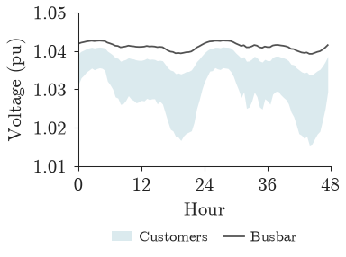
Over the two days, customer voltages range from 1.015 to 1.041 pu, all below the busbar, which is held near 1.04 pu by the transformer.

Convergence

A time-series solve can fail to converge at some steps, most often when many inverters run a Volt-VAr control loop. OpenDSS still reports a solution at those steps, so the report records how many steps diverged.

report.converged, report.diverged_steps, report.total_steps

(True, 0, 96)

At a diverged step, each recorded customer voltage is NaN. To stop a study when any step diverges, call require_convergence(), which raises ConvergenceError.

Penetration sweeps

run_uk_sweep() and run_us_sweep() run a grid of EV and PV penetration levels on one feeder. Each scenario builds a fresh circuit from the same seed, so the customers who have PV at 40 % penetration still have it at 60 %. A sweep on this feeder takes several minutes, so it is not run on this page; the time series tutorial runs one.

Limitations

• The step length is fixed for a run, 30 minutes by default. Shorter events, such as a cloud passing, are averaged out.

• A bus’s recorded voltage is the mean across its connected phases. For a single-phase customer that is the voltage it sees; for a three-phase bus it hides any imbalance between phases.

• The solver iterates the inverter control loop up to 200 times per step by default. A step that needs more is reported as diverged; raise max_control_iterations only after checking why.