Signals
Much of the analysis of the meters of a low-voltage network describes what they have recorded, namely the groups of customers, the similar cases and the anomalous readings. A forecast must instead state a quantity that has not yet been observed, from what is known when the statement is made. In a distribution network the quantity may be the demand of a household, the generation of a roof or the charging of a vehicle. It may also be the load and the voltage that these produce together. The operator acts on the statement before the outcome arrives, so the value of a forecast is the quality of the decision that it allows [1].
The theory of time-series forecasting is established [2], [3], but the Low Voltage (LV) network changes what the theory has to explain. The series are short and irregular, and they sum too few loads for the behaviour of individual customers to average out. A method that is adequate for a region therefore cannot be assumed to transfer to a transformer or to a household. A conclusion that is stated without the truth that it should recover cannot say how far a forecast lies from the best that the information allows.
Three questions have to be settled before a forecaster is chosen. The first is what can be forecast from the information available at the origin, and what limits the accuracy. The second is how much of a series can be explained, and by which inputs. The third is how a forecaster is evaluated, so that a conclusion remains valid under the variation of training. This chapter answers the first and second questions. It formulates forecasting as a learning problem and builds a population of series whose truth is known. That population tests how a series is characterised, how much of it can be forecast and which inputs explain it, before any model is fitted. Chapter 2 answers the third question by comparing the families of forecasters and the protocol that separates them, and Chapter 3 extends the evaluation to probabilistic forecasts.
For the power-system reader, the chapter shows how to state the floor that the information sets on the error. It also shows how to measure how much of a load can be explained and how to select inputs without leaking the future. For the machine-learning reader, it states the learning problem formally and links each tool to the property of the load that it measures. It also shows why a conclusion drawn on a region does not transfer to a transformer or a household. Each equation is read in words and units, each method is shown on a real signal, and each result is followed by its meaning for the operator.
Forecasting in LV Networks
An operator forecasts in order to decide, and the decision fixes what is forecast, how far ahead, and how accurate the forecast has to be.
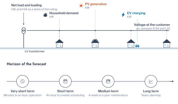
An LV network is a set of customers behind one distribution transformer, and an operator forecasts several of its quantities (Figure 1.1). Three of them belong to a customer, namely its demand, its generation and its charging. The demand \(y^{\mathrm{d}}_t\) is the energy that a household consumes in period \(t\). The generation \(y^{\mathrm{pv}}_t\) is the output of its photovoltaic array, and the charging \(y^{\mathrm{ev}}_t\) is the power that the charger of a vehicle draws. Their combination is the net load that the customer presents to the network,
\[ y^{\mathrm{net}}_t = y^{\mathrm{d}}_t + y^{\mathrm{ev}}_t - y^{\mathrm{pv}}_t, \tag{1.1}\]
which is positive when the customer draws power and negative when it exports. Two further quantities belong to the network, and the loading of a transformer is the net load of its \(N\) customers, \(y^{(N)}_t = \sum_{i=1}^{N} y^{\mathrm{net}}_{i,t}\), as a share of its rating. The voltage at a customer follows from the flows along the feeder and so depends on the same quantities. The forecast of the voltage and of the reactive power at a substation, besides the active power, supports the resilience of the network [4]. The target \(y_t\) of the rest of the part stands for any of these quantities, and the net load serves as the example because it combines the others.
The energy literature classifies forecasts by horizon into four classes [2], [3]. The very short term spans minutes to an hour, the short term an hour to a week, the medium term a week to a year, and the long term years. Each class serves a different decision of the distribution operator.
The very short term serves operation: it ranks the violations that are developing and decides whether a customer is curtailed or a tap changed. The short term serves scheduling, such as the day-ahead plan for charging and for flexibility offered to the market. It also serves new market players, such as aggregators and prosumers, in bidding, tariff design and storage scheduling [5]. The medium term serves maintenance and the outage plans that depend on the seasons. The long term serves planning, such as the hosting capacity of a feeder and the timing of reinforcement. The accuracy that a decision needs differs with the horizon, so the same error measure cannot serve an operator who acts within the hour and a planner of ten years.
The decisions above act on series that are hard to forecast, and the difficulty grows from the region to the household. A region sums thousands of customers whose appliances switch independently, so its daily cycle is stable. A transformer sums tens of customers and a household is one, so the behaviour of individual customers dominates and the series is irregular [6]. Few aggregated demand profiles and volatile generation from renewable sources make net-load forecasting at the LV level harder than at the transmission level [7]. Figure 1.2 measures the effect with the daily naive forecast, which repeats the load of the previous day [8], on five real signals. The median daily error is 15% of the mean load for a transformer of 18 customers and 76% for one household. No day of the transformer exceeds half the mean load, whereas 87% of the days of the household do. The household is from the AusNet study at half-hourly resolution and the transformer is from Porsgrunn at hourly resolution, so the two are not like for like. On the Porsgrunn customers alone, at one resolution, the error of the same forecaster is 0.42 of the mean load for one customer and 0.14 for 20 (Figure 1.18). A method that is adequate for a transformer therefore cannot be assumed to transfer to a household, and Problem Formulation and Notation states why the error falls as customers are added.
Three further properties separate the LV network from the transmission system, and each makes the load harder to forecast from its own history. Rooftop Photovoltaic (PV) turns a demand series that is always positive into a net load that is negative at midday, whose spread follows the irradiance and whose percentage error is undefined. Charging of electric vehicles adds rare, large and late blocks of load, at times that depend on the owner and not on the cycle of the day [9]. The records are short, subject to faults, and change as adoption grows, so a model fitted on last year describes a network that no longer exists. The effect of temperature, which is well established for a region, has to be reassessed at the LV level [10].
Figure 1.3 shows two forms of one household. Without generation and charging its demand is a series of spikes above a low base, with an evening peak whose height varies from day to day. With a 2.4 kWp array and a recorded vehicle the net load crosses zero at midday, when the array exports. It rises to about nine kilowatts when the vehicle charges in the evening. The first series requires the forecast of when the spikes occur. The second also requires the forecast of the weather, which sets the export, and of the behaviour of the owner, which sets the charging. Both depend on information that the history of the series does not hold. The choice of inputs and the design of the evaluation thus matter more here than the choice of model.
Remark: data that cross a boundary
The forecast of a transformer needs the sum of the meters behind it and the readings of no single customer. An operator that cannot release household readings can still forecast at the transformer. It keeps the household models within its own systems and shares only the forecast and its error.
The difficulty of forecasting in the LV network is consequently a matter of how little of the load the information at the origin can explain. Problem Formulation and Notation states that limit formally and shows how it falls as customers are summed.
Problem Formulation and Notation
Information and Irreducible Error
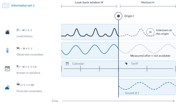
A forecast of one of these quantities is made at an origin \(t\) for the periods \(t+1, \dots, t+H\), where \(H\) is the horizon. It may use only the information set \(\mathcal{I}_t\) available at the origin,
\[ \mathcal{I}_t = \{\, y_{t-W+1:t},\; \mathbf{u}_{t-W+1:t},\; \mathbf{c}_{t-W+1:t+H},\; \hat{\mathbf{w}}_{t+1:t+H|t} \,\}. \tag{1.2}\]
The first element is the history of the series over a look-back window of \(W\) periods. The second, \(\mathbf{u}\), holds the covariates observed in the past, such as the measured temperature or the readings of other meters. The third, \(\mathbf{c}\), holds the inputs known in advance for the periods to be forecast, such as the calendar and the tariff. The fourth, \(\hat{\mathbf{w}}\), holds the forecasts of covariates, such as the weather forecast issued at the origin. A covariate observed only after the origin does not belong to \(\mathcal{I}_t\), and its use leaks the future [2], [11]. Figure 1.4 shows the four inputs on one time axis.
A forecaster is a function \(f_\theta\) with parameters \(\theta\) that maps the information set to the forecast,
\[ \hat{y}_{t+h|t} = f_\theta(\mathcal{I}_t), \qquad h = 1, \dots, H. \tag{1.3}\]
A loss \(\ell(y, \hat{y})\) measures the cost of one error, and the risk of a forecaster is its expected loss, \(R(f) = \mathbb{E}\,[\ell(y_{t+h}, f(\mathcal{I}_t))]\). Learning chooses \(\theta\) to minimise the empirical risk, the mean loss over the origins of a training period [12]. The evaluation measures the loss over later origins, because a random split lets the model see the future of the periods on which it is tested [13], [14].
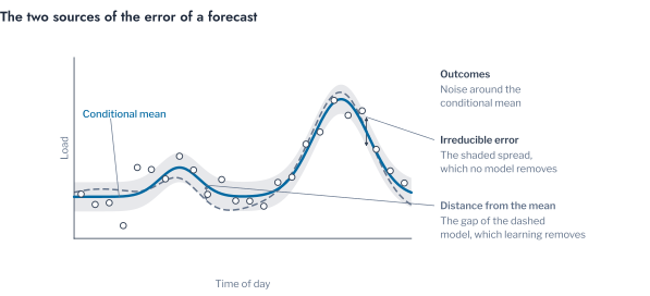
For the squared loss the minimiser of the risk is the conditional mean, \(f^{*}(\mathcal{I}_t) = \mathbb{E}\,[y_{t+h} \mid \mathcal{I}_t]\) [15], [16], and its risk is the expected conditional variance,
\[ R(f^{*}) = \mathbb{E}\,\big[\operatorname{Var}(y_{t+h} \mid \mathcal{I}_t)\big]. \tag{1.4}\]
This risk is the irreducible error: no model fitted to the information set can fall below it, and a better model can only approach it. The error of a forecaster accordingly has two sources. One is the distance of the model from the conditional mean, and the other is the variability that the information set leaves unexplained. The second source is the one that the LV network enlarges. Figure 1.5 shows the two sources on one day.
Remark: the irreducible error as a reserve
The irreducible error is the part of the load that no forecaster can remove, and it is what a reserve or a margin has to cover. A better model shrinks only the other part, the distance from the conditional mean. Once that distance is small, further tuning of the model yields no further gain.
Aggregation and Smoothing
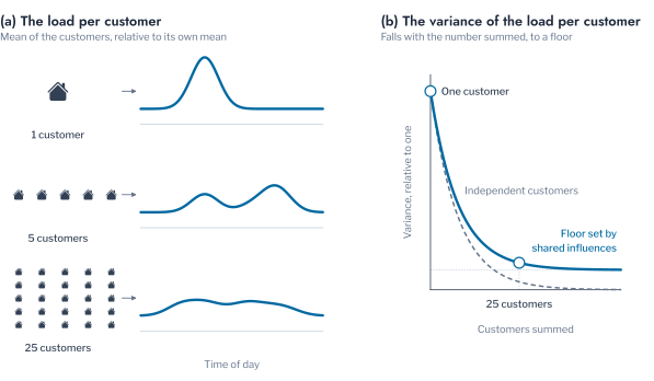
The unexplained variability of a household is larger than that of a region, which Figure 1.2 shows on real records, and Equation 1.4 gives the reason. Write the part of the load of customer \(i\) that the information set does not explain as \(\varepsilon_{i,t}\), with variance \(\sigma^2\) and a pairwise correlation \(\rho\) between customers. The mean over \(N\) customers has the variance
\[ \operatorname{Var}\Big(\frac{1}{N}\sum_{i=1}^{N} \varepsilon_{i,t}\Big) = \sigma^2\,\frac{1 + (N-1)\rho}{N}. \tag{1.5}\]
When customers behave independently, \(\rho = 0\), the variance falls as \(1/N\), so a region of thousands of customers is smooth and a household is not [6], [17]. When customers share an unexplained influence, such as a weather change that the forecast missed, \(\rho > 0\) and the variance cannot fall below \(\sigma^2 \rho\) however many customers are added. A region is therefore easier to forecast than a transformer of tens of customers, and a transformer is easier than a household. The floor of the variance is set by the shared influences. Figure 1.6 draws the idea. One customer is a sharp peak at its own time, the mean of five is lower and broader, and the mean of twenty-five is nearly flat. Assessing Forecastability measures the effect on the Porsgrunn customers.
The floor has a practical meaning for the operator. A forecast of a transformer cannot be improved below \(\sigma^2 \rho\) by a better model, because the shared influences are not in the information set. Money spent on a larger model is then better spent on the shared influence itself, such as a forecast of the weather, or on a reserve that covers what remains. The correlation \(\rho\) is therefore the first quantity to estimate for a group of customers, before any model is chosen. Assessing Forecastability shows how it can be read from the series.
Target and Horizon
The conditional mean is the point forecast, and the whole conditional distribution is the probabilistic forecast. An operator needs the second when a decision depends on the shape of the distribution, such as a reserve set at a stated probability [5]. Chapter 3 treats it, and Series of Known Truth generates series from a distribution that is known exactly.
The quantities of the network differ in the support and the shape of their distribution. Demand is positive, generation is zero at night and bounded by the clear-sky output, and charging is intermittent. The net load changes sign, and the voltage stays near one per unit. The loss and the evaluation measure thus depend on the target, and other losses give other targets, such as the quantiles of Chapter 3 [16]. The decomposition of the error holds for each of them.
Two choices remain once the problem is stated, what to forecast and how to produce the horizon. The net load of Equation 1.1 can be forecast in two ways. The additive strategy forecasts the demand, the charging and the generation separately and combines them. The integrated strategy forecasts the net load directly from its own history and from the covariates that drive its parts [18], [19]. The additive strategy needs a measured series for every part, which generation behind the meter does not provide, and the errors of the parts add. Comparisons with several model families found the integrated forecast more accurate [20], [21]. This part consequently forecasts the net load directly and uses the parts as inputs where they are measured.
The learning problem above forecasts one lead time. An operator needs a horizon of \(H\) periods from the same origin, and the strategy that produces it decides where the error of the forecast accumulates. A model that can be solved in closed form shows how.
A forecaster for lead time \(h\) is a function \(f_h\) of the information set. The direct strategy fits a separate \(f_h\) for each lead time \(h = 1, \dots, H\). Each lead time is then a learning problem with its own risk, fitted on the pairs of an information set and the value \(y_{t+h}\). The recursive strategy fits one forecaster of the next period and applies it \(H\) times, replacing the unknown values in its input by its own forecasts. The multi-output strategy fits one model that returns the whole horizon at once,
\[ \hat{\mathbf{y}}_{t+1:t+H|t} = f(\mathcal{I}_t;\, \boldsymbol{\theta}), \tag{1.6}\]
and shares its parameters across lead times [22]. Figure 1.7 contrasts the first two on one evening. The direct forecast reaches each lead time from the origin. The recursive forecast hops from one forecast to the next and carries the error of each hop forward.
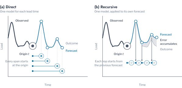
The effect is exact in the simplest model. Let \(y_{t+1} = \phi\, y_t + \varepsilon_{t+1}\) with independent noise and \(|\phi| < 1\). The conditional mean at lead time \(h\) is \(\phi^{h} y_t\). A recursive forecaster that has estimated \(\hat\phi = \phi + \delta\) forecasts \(\hat\phi^{\,h} y_t\), and its error against the conditional mean is, for small \(\delta\),
\[ \hat\phi^{\,h} y_t - \phi^{h} y_t \;\approx\; h\, \phi^{h-1}\, \delta\, y_t. \tag{1.7}\]
The single estimation error \(\delta\) is multiplied by the lead time, so it grows with \(h\) until the decay of \(\phi^{h-1}\) overtakes it. A load series with a daily persistence close to one accordingly accumulates the error almost linearly over a day. The direct strategy estimates the slope of each lead time separately, so the error of one slope does not enter another.
The comparison has a cost on each side. The recursive strategy is more efficient when the one-step model is correctly specified, because one estimate serves every lead time. The direct strategy is more robust to misspecification, because each model is fitted to its own lead time [23]. On 111 daily series the strategies that return the whole horizon at once were the most accurate [22]. The recursive strategy also needs future values of every past-observed covariate \(\mathbf{u}\). The operator does not have them for a measured temperature or for the readings of another meter. For the LV network the direct and multi-output strategies are therefore the default, and the recursive strategy is kept for models whose inputs are the series itself and the calendar.
Table 1.1 fixes the notation of the part. It keeps one symbol for one quantity: \(L\) is a limit, and the look-back window is \(W\).
| Symbol | Meaning |
|---|---|
| \(y_t\), \(\hat y_{t+h\mid t}\) | Target at period \(t\), which is any quantity of the network, and its forecast of lead time \(h\) made at origin \(t\) |
| \(W\), \(H\), \(h\) | Look-back window, horizon and lead time, in periods |
| \(y^{\mathrm{d}}_t\), \(y^{\mathrm{ev}}_t\), \(y^{\mathrm{pv}}_t\) | Demand, charging and generation, with net load \(y^{\mathrm{net}}_t = y^{\mathrm{d}}_t + y^{\mathrm{ev}}_t - y^{\mathrm{pv}}_t\) |
| \(N\), \(y^{(N)}_t\) | Number of customers behind a transformer, and the sum of their net loads |
| \(\mathbf{u}_t\), \(\mathbf{c}_t\), \(\hat{\mathbf{w}}_t\), \(\mathcal{I}_t\) | Covariates observed in the past, inputs known in advance, forecast covariates, and the information set |
| \(f\), \(\boldsymbol{\theta}\), \(\ell\), \(R\) | Forecaster, its parameters, loss and risk |
| \(\varepsilon_{i,t}\), \(\sigma^2\), \(\rho\) | Part of the load of customer \(i\) that the information set leaves unexplained, its variance and the correlation between customers |
| \(L\) | A limit |
The notation fixes what is forecast, the information that a forecaster may use and the error that no model can remove. Series of Known Truth builds a population in which that error is known exactly, so that every tool of the part can be checked against it. Some letters serve a single equation, such as the counts \(A\) and \(B\) of the sample entropy or the season length \(m\) of a decomposition. They are defined where they appear and are local to that equation.
Series of Known Truth
A forecast of a real series is scored against one realisation, so its score cannot say how close the forecast is to the best that the information allows. A measure of tail weight, a score or a significance test applied to a real series has the same weakness, because the truth that it should recover is unknown. This section therefore generates series from a conditional distribution that is known exactly. Every characterisation, score and test of the part is applied first where the answer is known.
Each synthetic series follows
\[ y_t = \mu_t + \sigma_t\, \varepsilon_t, \qquad \varepsilon_t \sim G, \tag{1.8}\]
where \(\mu_t\) is the median net load and \(\sigma_t\) the scale of the noise. The noise families are standardised to a zero median and an interquartile range of 1.349, so \(\mu_t\) is the location of the net load. The conditional mean equals \(\mu_t + \sigma_t\,\mathbb{E}[\varepsilon_t]\), and it differs from \(\mu_t\) only for a skewed family. The location is a double-peaked daily load with weekly and seasonal variation, minus the output of PV under clear-sky irradiance reduced by random cloud cover. Its peak is 20 kW, the order of a transformer with tens of customers, and PV is 40% of it. The noise \(\varepsilon_t\) is drawn by inverse transform, \(\varepsilon_t = G^{-1}(U_t)\) with \(U_t\) uniform, so the true conditional quantile of level \(\tau\) is
\[ q_\tau(t) = \mu_t + \sigma_t\, G^{-1}(\tau). \tag{1.9}\]
The forecaster that knows \(\mu_t\), \(\sigma_t\) and \(G\), the oracle, attains the irreducible error of Equation 1.4. Its expected loss under any strictly proper scoring rule is the lowest that any forecaster can reach [24]. The pinball loss at each quantile level has the true quantile as its minimiser [16], [25], so the oracle also attains the lowest pinball loss. The excess of the loss of a method over that of the oracle thus measures its distance from the best forecast, which a real series never provides.
Remark: the oracle
The oracle is the forecaster that knows the rule that generated the series, as a network model with exact data is an oracle for a power flow. It cannot exist for a real series, and it is built here to show what a method should reach and how far a real method falls short.
The families \(G\) are standardised to a zero median and the interquartile range 1.349 of the standard normal, so their bodies agree and only the tails and the shape differ. Figure 1.8 shows five of them against the normal. The Student-t density with three degrees of freedom has a long, symmetric tail, the skew-normal [26] and the lognormal are asymmetric, and the mixture has two modes. The twelve factors of the generator also vary the scale and the tails with the conditions. The scale of the noise rises with PV output from 0.72 kW at night to 5 kW at noon. The degrees of freedom of a Student-t fall or rise with the clear-sky profile. In one factor the noise changes family on a given date.
With the generator defined, one week of its output shows what the truth looks like. Figure 1.9 sets one week of four factors against the true 90% band of each step. The band is 5.9 kW wide for the Gaussian series. It is 7.5 kW wide for the Student-t series with three degrees of freedom. The body is the same, but the 5% and 95% quantiles lie further out in a heavy tail. The band of the heteroscedastic series is 2.4 kW wide at night and 16.1 kW at noon, and that of the mixture is 3.6 kW wide. A forecaster that reports a band of constant width is correct for the first series and too narrow for the second. It is wrong at both ends of the day for the third.
The points outside the band are the same 31 of 336 steps in every factor, 9.2%, because the factors share the uniform draws. What differs is how far they lie from the band. The largest excursion of the Student-t series is 9.4 kW and its mean is 2.5 kW, against 0.6 kW and 0.2 kW for the mixture. A measure that averages squared distances, such as the root mean square error, is consequently dominated by a few steps of a heavy-tailed series [27]. The comparison of forecasters in the sections on evaluation shows what that does to a ranking.
The generator accordingly supplies the truth against which the tools of the following sections are checked, beginning with the characterisation of a series in Characterising a Series.
Characterising a Series
Stationarity Tests
An operator who must choose a model first needs to know what the series allows. The daily naive forecast of Figure 1.2 serves a transformer and fails a household, and five properties of a series explain the difference. They are the drift of the level, the share that repeats each day, the reach of the history, the constancy of the spread and the speed of change. These properties are measured on five real signals, and the tools are then checked on series whose properties are known. The first signal is the demand of a median AusNet household, labelled Household in the figures. The second is the same household with a small array and a recorded vehicle, labelled Household, PV, EV. The third is the net load of an LV transformer of Porsgrunn. The fourth is the output of one PV array, labelled PV system, and the fifth is the charging of a car park at an assumed constant power, labelled EV charging. Each measure is computed on a training window of 4,000 observations, which is 83 days of half-hourly data or 167 days of hourly data. Nothing from the period to be forecast then enters the choice of the model.
The augmented Dickey-Fuller regression
\[ \Delta y_t = \alpha + \beta t + \gamma\, y_{t-1} + \sum_{i=1}^{p} \delta_i\, \Delta y_{t-i} + e_t \tag{1.10}\]
tests the null hypothesis \(\gamma = 0\), a unit root [28]. The KPSS statistic
\[ \eta = \frac{1}{T^{2}\, \hat\sigma^{2}_{\infty}} \sum_{t=1}^{T} S_t^{2}, \qquad S_t = \sum_{s=1}^{t} \hat e_s, \tag{1.11}\]
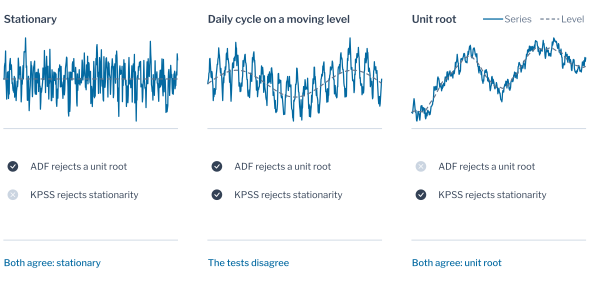
tests the reverse null hypothesis, stationarity around a level or a trend [29]. Read together, the two tests give four outcomes. The series is stationary when the first rejects and the second does not, and it is difference-stationary when the second rejects and the first does not. When both reject, the tests disagree, and the series has either a long memory or a deterministic structure that the regression does not remove.
A unit root would mean that a disturbance of the load never fades, so that lagged values are informative only as differences. The first test rejects a unit root for all five signals, with a p-value below 0.001, so disturbances fade in all of them. The second rejects stationarity for four, which means that their level still moves over the window, for instance with the season or the weather. It does not reject for the household with the array and the vehicle, whose p-value of 0.10 is the upper limit of the tabulated values. The four signals therefore fall in the case where the tests disagree, and the rule of the characterisation would difference them. The reading cannot separate a unit root from a strong daily cycle on a slowly moving level. The check on known truth below shows that the rule also differences series that have no unit root. Their lagged inputs are therefore given as differences or as deviations from the daily profile. Figure 1.10 shows the four outcomes of the two tests on three series.
Remark: a unit root and a seasonal level
A unit root means that the load has no preferred level, so a disturbance stays. A seasonal level means that the preferred level moves with the calendar and the load returns to it, as the mean load of a winter does. Over a few months of data the two look alike.
Seasonal Structure
Multiple seasonal-trend decomposition by loess separates the series into a trend, the seasonal components and a remainder [30],
\[ y_t = T_t + \sum_{k} S_t^{(m_k)} + R_t, \tag{1.12}\]
with the seasonal periods \(m_k\) of one day and one week. The strength of a component \(C\) is \(F_C = \max\bigl(0,\, 1 - \operatorname{Var}(R_t)/\operatorname{Var}(C_t + R_t)\bigr)\), the share of the variation that the component explains beyond the remainder [8], [31]. A value near 1 means that the component repeats almost exactly from one period to the next, and a value near 0 means that it does not repeat.
Figure 1.11 (a) gives the daily strength of each signal as the filled point and the weekly strength as the open point. The PV array repeats its day most, at 0.69, because the sun rises and sets every day, and the charging of the car park follows at 0.60. The transformer reaches 0.50 since it sums the routines of its customers, whereas a single household reaches only 0.39 and so varies its day more than a transformer does. The household with the array and the vehicle is the lowest at 0.34. Each of them adds a part that does not repeat from one day to the next, so the strength falls from 0.39 once they are added. Across all signals the weekly strength lies between 0.11 and 0.25. The periodogram agrees on the day, with its strongest period at 48 half-hours for the two households and at 24 hours for the PV array and the charging. For the transformer the strongest period is 12 hours and the second is 24 hours, so the half-day harmonic of the daily cycle is the stronger of the two.
The daily cycle is thus the main repeating structure of every signal, and the calendar of the day enters every model, whereas the day of the week matters less. No signal repeats its day by more than 0.69, and the transformer by 0.50. The rest of the variation has to come from other inputs. They are the weather for the PV array and the behaviour of the customers for the household and the charging.
Autocorrelation and Memory
The decomposition shows that the day repeats, and the autocorrelation shows how far the past informs the future. The autocorrelation at lag \(k\) is
\[ \hat\rho_k = \frac{\sum_{t=k+1}^{T} (y_t - \bar y)(y_{t-k} - \bar y)}{\sum_{t=1}^{T} (y_t - \bar y)^{2}}, \tag{1.13}\]
The autocorrelation is the correlation between the load now and the load \(k\) periods earlier [32]. It is 0 when the past carries no linear information and 1 when the load repeats exactly. Its square is the share of the variance that the earlier value explains. The partial autocorrelation removes the effect of the shorter lags, and the lag at which it stops being significant is a candidate for the autoregressive order. The peaks of the autocorrelation at multiples of a period give the seasonal periods [8]. The autocorrelation of an integrated series is high at every lag [33], so it is taken on the differenced series when the stationarity tests call for differencing. Both are shown below, because the verdict can call for differencing a series that has no unit root. The shortest significant peak sets the look-back window \(W\), as the shortest span over which the dynamics repeat. The longer peaks become candidates for lagged inputs, together with the half-period, and they are kept out of the window so that the inputs stay free of redundant lags (Figure 1.12).
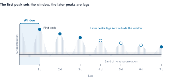
Figure 1.13 shows the autocorrelation of the transformer and of the household over seven days, in levels and in first differences. The autocorrelation of the transformer in levels (Figure 1.13 (a)) is 0.82 at one day, so the load of yesterday explains about two thirds of its variance. It is 0.77 at two days, 0.75 at three and 0.69 at seven. It stays far above the grey band that marks the absence of autocorrelation, which is \(\pm 1.96/\sqrt{T}\) [32]. One day is accordingly the window, and half a day, two days, three days and a week are lags to test. The household in levels (Figure 1.13 (c)) reaches only 0.19 at 2.1 days and 0.17 at seven, so its past explains about 4% of its variance at the lags marked. It is negative at half a day, where the load lies on the opposite side of the daily cycle.
The levels overstate how far the past informs the future, and the differences show by how much. On the differences (Figure 1.13 (b)) the transformer still repeats daily. Its autocorrelation is 0.24 at one day, 0.21 at two, 0.18 at three and 0.24 at seven, all above the band. The changes of its load repeat, but far less than its level does. The household keeps almost no structure in its differences (Figure 1.13 (d)). Their autocorrelation is 0.01 at half a day and at seven days and 0.06 at 2.1 days, which is slightly outside the band. The characterisation takes its peaks from the differences when they show any and from the levels otherwise, and its lags are candidates to be tested. The inputs beyond the series, the calendar and the weather, have to carry the forecast of a household. A short window of its own history serves for the transformer.
The order itself is not fixed by the series. The cutoff of the partial autocorrelation is taken on the differences where the tests call for them. It is 0 for the household and the transformer, 2 for the household with the array and the vehicle, 3 for the charging and 24 for the PV array. The criteria AIC [34] and BIC [35] choose the number of lags that balances the fit against the number of parameters, and BIC penalises the parameters more. BIC selects between 4 and 48 lags, and AIC selects the longest order tested for all five signals. The information criteria therefore do not settle the order either. The window comes from the seasonal period and not from an autoregressive order, and the order is a screening choice.
The Ljung-Box statistic
\[ Q = T(T+2) \sum_{k=1}^{m} \frac{\hat\rho_k^{2}}{T - k} \tag{1.14}\]
tests that the first \(m\) autocorrelations are jointly zero [36]. Applied to the remainder of the decomposition with \(m\) equal to one day, it rejects for all five signals, with a p-value below 0.001. The remainder therefore shows autocorrelation that chance does not produce. The remainder is not white noise, and structure remains after the daily and the weekly cycle are removed, which a model with lagged inputs and covariates can use. The same statistic applied to the residuals of a forecaster checks whether the model has taken that structure.
Variance and Ramps
The remainder of the decomposition still carries structure, and its variance is the next property to test. The ARCH test regresses the squared remainder on its own lags [37],
\[ \hat e_t^{2} = \alpha_0 + \sum_{i=1}^{q} \alpha_i\, \hat e_{t-i}^{2} + v_t, \tag{1.15}\]
and rejects a constant variance when \(T R^{2}\) exceeds the critical value of the \(\chi^{2}_q\) distribution. A constant variance would mean that the uncertainty of the load is the same at every hour. The test rejects for all five signals, with a p-value below 0.001. The remainder thus holds structure that the decomposition has left, and the check on known truth below shows how far a rejection says that the noise scale changes. The BDS test asks whether the remainder retains dependence that no linear model can describe [38], and it rejects for all five. A nonlinear model can consequently use dependence that a linear one leaves in the remainder.
The spread and the level of a signal can also change from one day to the next. The lumpiness is the variance of the variances of the daily windows of the standardised series, so it is high when the spread changes [39]. The stability, in turn, is the variance of the means of the same windows and is high when the level moves [39]. The transformer has the steadiest spread, with a lumpiness of 0.02, and the PV array the least steady, at 2.95, as expected of an output that follows the sun. The household with the array and the vehicle follows at 0.80. In level the transformer moves most between days, with a stability of 0.77 against 0.08 for the household. A model of the PV array and of the household with PV and EV accordingly has to model the spread. A model of the transformer has to follow its level, so inputs that move with the weather and the season matter for it.
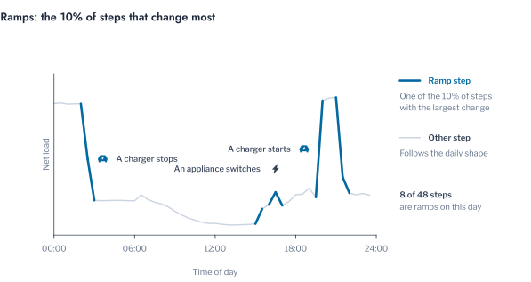
A step is a ramp when its absolute first difference lies among the largest 10%. It is where an appliance switches, a charger starts or a cloud passes over an array. The sample entropy measures how often a pattern of recent values that repeats is followed by a similar next value, so it is higher for a less regular series. It is 0.03 to 1.0 on the other steps and 1.5 to 2.1 on the ramps. The PV array is almost perfectly regular outside its ramps, at 0.03, and 58 times as irregular on them. The transformer and the charging are about twice as irregular on the ramps. The value after a ramp therefore depends little on the pattern before it. The errors of a forecaster concentrate there, at the steps that matter most to an operator who watches a limit. Figure 1.14 marks the ramps of one day. A model fitted on all steps averages two kinds of behaviour, so the error of a forecaster is reported separately for the ramps and for the other steps.
Checking Against Known Truth
The tools above report what they see, and the population of Series of Known Truth shows whether they see what is there. Figure 1.15 applies them to the twelve factors over three years each, where the cycle, the stationarity and the noise are known. The periodogram finds the day on every factor, with its strongest periods at 24 and 48 steps, the half-day harmonic of the double-peaked daily load and the day itself. The stationarity tests disagree on all twelve, with a p-value below 0.001 for ADF and 0.01 for KPSS. None of them has a unit root, since the only drift is the annual cycle of the mean. The rule that differences a series when the tests disagree would therefore difference all twelve. A disagreement is a flag to compare inputs in levels and in differences, and not a verdict.
The ARCH statistic of the remainder of the decomposition (Figure 1.15 (a)) exceeds the 5% critical value of 65 for all twelve factors, including the eight whose noise scale is constant. The remainder holds the variation of the cloud cover that the decomposition leaves. Only the series whose scale follows the sun stands apart, at 9,458 against at most 1,744. Applied to the true noise, the test rejects only that series, and it misses both the tails that change with the hour and the change of scale in 2021. A rejection on a real signal thus shows that the remainder is structured, and the size of the statistic against a reference series says more than its p-value. The lumpiness of the daily windows (Figure 1.15 (b)) is 0.74 to 0.88 for the three factors with the heaviest tails. It is at most 0.07 for the others, so it finds heavy tails and not changes of scale. The household has a lumpiness of 0.40 over its training window and the household with the array and the vehicle 0.80. Both lie among the heavy-tailed series and far above the 0.07 of the rest.
The record of a series can also change. The production meter of the PV array shows no output for the first 238 days, so a forecaster fitted on the whole record would average two different series. A cumulative sum of recursive residuals flags such a change of normal behaviour [40]. The training window of this section starts at the first reading of the array for that reason.
To characterise a new series, follow these steps, using nothing after the end of a training window.
- Run both stationarity tests and treat a disagreement as a flag, giving the lagged inputs as differences or as deviations from the daily profile.
- Read the strength of the daily component to see how much the calendar can carry, and take the period from the periodogram.
- Set the window from the shortest period, and take the lags from the longer peaks of the autocorrelation, in levels and in differences.
- Test the remainder with the Ljung-Box statistic, read the ARCH statistic against a reference series, and check the lumpiness for heavy tails.
- Report the error of a forecaster separately for the ramps and for the other steps.
Pitfall: characterising a series on its levels
A series that is integrated shows a high autocorrelation at every lag, so every lag looks informative and the characterisation suggests a long window [33]. Test for stationarity first, and take the autocorrelation of the differences when the tests call for them.
The characterisation says what a series is: how it repeats, how far its past informs and where it changes quickly. Assessing Forecastability turns those properties into a measure of how much of the series can be explained.
Assessing Forecastability
Nine Forecastability Measures
A household forecast by the daily naive rule errs by a median of 76% of its mean load, against 15% for a transformer (Figure 1.2). Whether a better model could bring the household down to 20% depends on how much of its load can be forecast at all. The error of one forecaster does not say. That share is the forecastability of the series, and it is measured here in three steps. It states measures that are computed from the series alone, tests them on series whose answer is known, and then reads the real signals through that test.
Nine measures are used, and each asks one question. Over a year the household has the daily strength of Characterising a Series of 0.44 and the transformer 0.55, which says what share of the variation repeats from day to day. The linear predictability is the share of the variance that an autoregression of order \(p\) explains,
\[ R^{2}_{p} = 1 - \frac{\hat\sigma^{2}_{e}}{\hat\sigma^{2}_{y}}, \tag{1.16}\]
the linear bound of what the past gives one step ahead. It is 0.60 for the household and 0.94 for the transformer. The spectral forecastability of Goerg is estimated from the share \(p_k\) of the power of the series at each of the \(K\) Fourier frequencies,
\[ \hat\Omega(y) = 1 - \frac{-\sum_{k=1}^{K} p_k \log p_k}{\log K}, \tag{1.17}\]
one minus the normalised entropy of the spectrum [41]. The spectrum is estimated by averaging the periodograms of segments of the series [42]. The estimate lies between 0 and 1: it is 1 for a sinusoid, with its power at one frequency, and 0 for white noise, with its power spread evenly. It is 0.19 for the household and 0.25 for the transformer.
Two entropies ask how regularly a series repeats its patterns. The sample entropy is
\[ \mathrm{SampEn}(m, r) = -\log \frac{A}{B}, \tag{1.18}\]
where \(B\) counts the pairs of sequences of \(m\) values that stay within a tolerance \(r\) of each other and \(A\) counts those that still do with \(m+1\) values [43]. The permutation entropy
\[ \mathrm{PE}_d = -\frac{1}{\log d!} \sum_{\pi} p(\pi) \log p(\pi) \tag{1.19}\]
measures the regularity of the ordinal patterns \(\pi\) of order \(d\) [44]. Both are low for a series that repeats. The exponent \(\alpha\) of detrended fluctuation analysis, defined by \(F(n) \propto n^{\alpha}\) [45], and the Hurst exponent [46] ask whether fluctuations persist. A value below 0.5 means that they reverse, 0.5 means that they have no memory, and a value above 0.5 means that they persist.
The coefficient of variation asks how large the variation is against the mean, so it measures difficulty and not predictability. The skill of yesterday is
\[ \mathrm{SS} = 1 - \frac{\mathrm{MAE}_{\text{yesterday}}}{\mathrm{MAE}_{\text{mean day}}}, \tag{1.20}\]
the gain of a forecast that repeats the previous day over one that repeats the mean day, scored on the second half of the series. It is positive only when the deviation of a day persists into the next, and it is about \(1 - \sqrt{2}\) for a repeating cycle with independent noise. It is \(-0.13\) for the household and 0.69 for the transformer. The information that the past holds at each lead time is the auto-mutual information of the differences,
\[ \mathrm{AMI}(h) = I(\Delta y_{t+h};\, \Delta y_{t}), \tag{1.21}\]
estimated from nearest neighbours [47]. It captures nonlinear dependence, and it is taken on the differences because persistence inflates it on levels. Its effective horizon is the first lead time at which it falls to the noise floor.
Reading Real Signals
Figure 1.17 (a) reads the five real signals through the calibration with three measures. The household reads 0.45, 0.67 and 0.67 from the daily strength, the linear predictability and the spectral forecastability. The household with the array and the vehicle reads 0.36, 0.73 and 0.73. The transformer reads 0.59, 0.98 and 0.79, the PV array 0.86, 0.94 and 0.98, and the charging 0.67, 0.86 and 0.92. All three measures put the two households lowest and the other three signals above them. The readings of a signal differ by 0.12 for the PV array and by 0.39 for the transformer. The spread between the measures, and not the error of the calibration, is therefore the uncertainty of a reading. The daily strength is the most cautious of the three. It counts only the part of the load that repeats from day to day, whereas the other two also count the persistence from one period to the next.
The 342 AusNet households, read from the linear predictability, have a median share of 0.64. Half of them lie between 0.57 and 0.71, and the range is from 0.34 to 0.92, with every reading inside the range of the calibration (Figure 1.17 (b)). Most households can thus be explained to about two thirds of their variance. The household at 0.34 has two thirds unexplained by a model that uses the calendar and the weather. An operator can screen the meters of a programme with a year of readings and put the low ones behind an aggregate. The skill of yesterday has a median of \(-0.11\) over the households. For more than half of them the previous day is a worse guide than the mean day. A forecast that repeats yesterday is consequently not a safe benchmark for a household, and the baseline has to be chosen for each one.
Aggregation and Horizon
Aggregation raises the reading in the same way. On the Porsgrunn customers the spectral forecastability of the aggregate, read through the hourly calibration, gives 0.65 for one customer. It gives 0.79 for 10, 0.86 for 20, 0.95 for 100 and 0.98 for 1,000. The value of 0.48 for all 4,215 customers lies above the range of the calibration, so its reading of 0.99 is an extrapolation. The reading of 0.65 for one Porsgrunn customer agrees with the 0.67 of the AusNet household, which is a check on the calibration between two populations. Figure 1.18 shows the curves themselves. The error of the daily naive forecast is 0.42 of the mean load for one customer, 0.18 for 10 customers, 0.14 for 20 and 0.085 for 100. It flattens at 0.062 for 1,000 customers and 0.058 for all 4,215. The flattening is the floor of Equation 1.5, since the influences that all customers share remain however many are summed. Summing 20 customers lowers the error of the same forecaster by two thirds before any change of model.
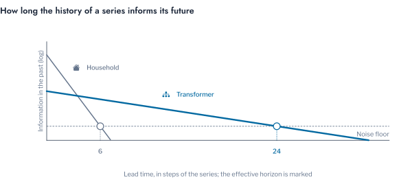
The share says how much of a series can be explained, and the auto-mutual information says for how long its own history helps. The auto-mutual information of the five signals of Characterising a Series is low for all of them. At one step it is 0.28 nats for the household and 0.24 for the household with the array and the vehicle. It is 0.15 for the charging, 0.22 for the PV array and 0.05 for the transformer. The effective horizon is 4 half-hours for the household, which is 2 hours, and 6 half-hours for the household with the array and the vehicle, which is 3 hours. It is 2 hours for the charging, 7 hours for the PV array and 22 hours for the transformer. A forecast further ahead than that has to rest on the calendar and the weather, and not on the history of the series. Figure 1.19 draws the two cases.
Agreement of Measures
Figure 1.20 shows how the nine measures agree over the 342 households (Figure 1.20 (a)) and over the 96 series of known truth (Figure 1.20 (b)), on one order and one scale. The rank correlation of two measures is +1 when they order the series alike and \(-1\) when they order it in reverse. A higher entropy or coefficient of variation means a harder series, so these three measures are reversed first, and a positive value then always means that two measures agree. On the households the linear predictability and the spectral forecastability agree most, at 0.93. The daily strength agrees with them at 0.45 and 0.63, and the fluctuation exponent at 0.61 and 0.50. The entropies and the Hurst exponent relate weakly to those four, at most 0.29 in absolute value, and the sample entropy relates to the coefficient of variation at \(-0.65\). The Hurst estimate leaves the range from 0 to 1 for at least one household, where it is \(-3.99\). On the known truth, in contrast, five measures agree at 0.99 or more. They are the daily strength, the skill of yesterday, the fluctuation exponent and the two variance measures. The coefficient of variation, reversed, agrees with them at 0.98 to 0.99. The series there differ only in the share of their noise. The households differ in more ways than that, so the agreement on the known truth is an upper bound, and the ranking of households depends on the measure. The readings above accordingly use the variance measures that the known truth supports, and they compare their agreement on each signal.
Remark: the explainable share and the margin
The explainable share is the part of the variance that a model using the calendar and the weather can remove. The rest is the error that an operator accepts or covers with a margin, so the reading of a signal sets how wide a margin its forecast needs.
To apply the measures to a new series, follow these steps.
- Take at least a year of the series at its own resolution.
- Compute the daily strength, the linear predictability and the spectral forecastability, and read each through the calibration of the same resolution.
- Rely on the reading when the three agree, and take the daily strength as the cautious value when they differ.
- Compare the reading with the error of the best forecaster fitted. An error far above what the reading allows means that the model is the limit and not the series.
Pitfall: one measure read as forecastability
Each measure sees one kind of structure, and the entropies and the Hurst exponent do not follow the known truth. Read several variance measures together, compute them on the differences when the levels are integrated, and compute them on the ramps and on the other steps separately, as in Characterising a Series. Entropy and auto-mutual information taken on levels measure persistence.
A series that can be explained to about two thirds of its variance still needs inputs that carry the explanation. Which candidates those are, and whether each adds to the others, is the question of input selection.
Input Relevance and Selection
Six Relevance Measures
Every input that a model reads adds a column to it, and an input without information adds error. It also costs the operator the purchase, archiving and checking of the forecast that feeds it. The previous section measured how much of a series can be explained, and the question now is which inputs explain it. The candidates are the past of the load, the calendar and the weather. The calendar is known for every step of the horizon, and the weather is observed in the past and forecast ahead. The choice is tested on the Porsgrunn transformer of 18 customers, with ten weather variables, hourly from 1 January 2022 to 30 September 2024. The record has 336 missing hours, which are left empty on a regular hourly grid, so that every lag is a true shift in time. It is also tested on the series of known truth of Series of Known Truth, where the irradiance drives the load. The temperature of those series follows the season but does not drive the load, and a column of noise has no relation to it.
The relevance of an input is the dependence between that input and the load, measured on the input alone. The benefit of an input is the reduction of the error of a forecaster that already uses the other inputs. The first needs no model and the second does, so the relevance ranks the candidates and the benefit decides.
Six measures of relevance are used, and each sees one kind of dependence. The rank correlation \(\rho_S\) [48] sees any monotone relationship. The F statistic of a regression of the load on the input equals the share \(R^{2} = F/(F + n - 2)\) of the variance that a line explains, so it sees a linear relationship only. The distance correlation [49] is zero only when the input and the load are independent, whatever the form of the relationship. The mutual information
\[ I(X;Y) = \mathbb{E}\left[\log \frac{p(x,y)}{p(x)\,p(y)}\right] \]
is also zero only under independence. It is estimated from the nearest neighbours of each observation [47]. Chatterjee’s coefficient takes the ranks \(r_i\) of the load with the pairs ordered by the input, and without ties it is
\[ \xi_n = 1 - \frac{3\sum_{i=1}^{n-1} \lvert r_{i+1} - r_i \rvert}{n^{2} - 1}, \]
which approaches 1 when the load is a function of the input and 0 under independence [50]. The predictive power is one minus the ratio of the error of a small decision tree to that of the median, and it sees whatever a tree can learn1. The impurity-based importance of a forest [51] is each input’s share of the total fall in impurity over the trees, and it needs several inputs.
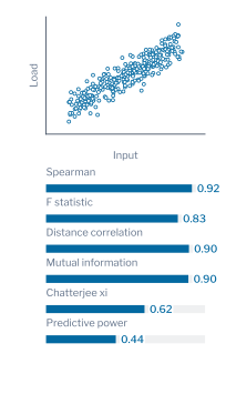
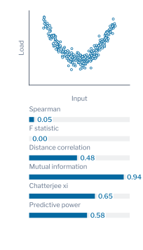
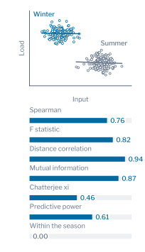
Figure 1.21 shows how the measures divide on three relationships. On a monotone relationship (Figure 1.21 (a)) all of them score the input. A U-shaped relationship (Figure 1.21 (b)) arises when a load rises as the temperature departs from a comfortable value in either direction. There the rank correlation is 0.05, the F statistic 0.00 and the mutual information 0.94. A ranking that used only linear measures would discard an input that is strongly related to the load. In the third relationship (Figure 1.21 (c)) the input and the load both follow the season. Every measure scores the pooled data high, with a rank correlation of 0.76 and a distance correlation of 0.94, yet xi within each season is zero. The dependence is real in the data and disappears once the season is known. A temperature that rises and falls with the season behaves partly in this way.
Fusing the Rankings
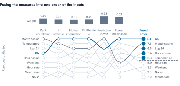
The six rankings differ, so they are fused. Each input receives its rank under each measure, and the ranks are added with a weight for each measure,
\[ s_j = \sum_{m=1}^{6} w_m\, r_{jm}, \qquad w_m \propto \max\left(0.05,\; 1 - \overline{\lvert \rho_S(m, m') \rvert}\right), \]
where \(r_{jm}\) is the rank of input \(j\) under measure \(m\), larger for a more relevant input, and the bar is the mean over the other measures. A measure that repeats the others counts less, which is the rule of a weighted Borda count [52]. The geometric mean of the ranks is an alternative that penalises an input ranked very low by one measure. The reciprocal rank fusion [53] is another, and it gives the top ranks the most weight. On the known truth the unweighted sum, the weighted sum, the arithmetic mean and the geometric mean give the same first three inputs. They differ only among the neighbours below, where the hour cosine and the temperature exchange the fourth and fifth places. The choice among them therefore matters little when the measures broadly agree.
Figure 1.22 reads the nine candidates on the first 12 months of the synthetic series. That is the first training window of the comparison in Chapter 2, so the ranking sees none of its test windows. The four dependence measures have weights from 0.13 to 0.16. The predictive power and the forest, which rest on a model and repeat the others least, have 0.23 and 0.21. The irradiance is first and the noise is among the last two, which is the right order at both ends. The temperature, however, is fifth, so a cut at five inputs keeps it although it does not drive the load. Its rank correlation of 0.58 exceeds the 0.51 of the irradiance because it follows the season. Its predictive power, however, is 0.00 against 0.10, and its forest importance is 0.07 against 0.43. The measures that rest on a model thus separate two inputs that the dependence measures do not. A ranking by relevance alone cannot be trusted to remove an input that the season carries along.
Remark: marginal relevance and conditional benefit
A measure of relevance scores an input alone, so it is a marginal quantity. The benefit of an input is conditional on the inputs already in the model, as the partial effect of a regressor is conditional on the others. Two inputs that carry the same information are each relevant and together worth one.
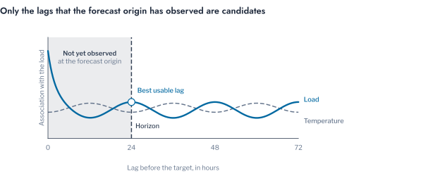
Lags and Information
The past of the load enters as lags, and a lag is admissible only if its value exists at the origin. A direct forecast of horizon \(H\) steps may use \(y_{t-h}\) for the target \(y_t\) only when \(h \ge H\) (Figure 1.4). Every lag shorter than the horizon is consequently removed before any scoring, whatever its score (Figure 1.23). The association of an input with the target at each admissible lag is the cross-lag profile \(\xi_n(x_{t-h}, y_t)\). On the first 8,000 hours of the Porsgrunn transformer the association of the load with its own past is 0.567 at 24 hours and 0.539 at 48 hours. It is 0.528 at 72 hours and falls to 0.437 at 36 hours, between the daily multiples. The daily multiples are accordingly the candidate lags, and the best usable one is the day before the target, which the daily naive forecast of Characterising a Series also uses. The temperature stays between 0.42 and 0.53 across the lags, and the solar radiation below 0.10. A slow input is used at the target hour as a forecast, and its own lags add little. The solar radiation relates weakly to the demand of this transformer.
On the Porsgrunn transformer the same six measures have weights between 0.14 and 0.16, except 0.25 for the forest. Their fusion ranks the load of the previous day first, the feels-like temperature second, the month third and the temperature fourth. The dew point follows in fifth place, the pressure in sixth and the solar radiation in eighth. The ranking uses the hours of 2022 only, which are the first training window of the comparison in Chapter 2. The column of noise is sixteenth of seventeen, above only the weekend. The order is plausible for a load that follows the outdoor temperature. It keeps three inputs that move with the same air mass, the temperature, the feels-like temperature and the dew point. The ranking cannot say how many of them the model needs.
The ranking is a shortlist and not a verdict. To rank the inputs of a new forecaster, follow these steps.
- List the candidates in the three families and fix the horizon.
- Remove the lags shorter than the horizon, and encode every cyclic calendar variable by a sine and a cosine [8].
- Score the candidates under the six measures on a random sample of a few thousand hours and fuse the ranks.
- Keep one of each group of inputs that repeat one another, and pass the shortlist to the test of benefit in Chapter 2.
Pitfall: a ranking read as a benefit
A high relevance means that an input carries information about the load, not that it adds to the inputs already present. An input that follows the season, or that repeats the calendar, ranks high and adds nothing. Decide by the skill of the set on windows of every season, which Chapter 2 measures.
The shortlist is the result of this chapter for the inputs. On the Porsgrunn transformer it holds the load of the previous day, the temperature and the calendar. Chapter 2 measures what each of them adds once the forecasters and the protocol of a comparison have been stated.
Further Applications
A method that has been checked on one transformer is useful only if it carries to the problems that an operator meets next. The tools of this chapter apply to several of them, and each changes one choice, the quantity, the horizon or the information set, while the method stays the same.
The first is the screening of customers by forecastability before a programme relies on their forecasts. A flexibility offer from a household is worth only as much as the household can be forecast. The measures of Assessing Forecastability rank the customers by it without fitting a model. The second is the choice of weather inputs and sensors. The relevance analysis of Input Relevance and Selection ranks the variables, and the test of benefit of Benefit of Input Sets says which of them repays its purchase. A third is the record of a transformer as an early signal of change. The characterisation of Characterising a Series, repeated on successive years, shows when the share of the daily cycle falls or the ramps grow as PV and charging are adopted. Detectors of change in a series can use that signal.
A fourth is the forecast of the charging of electric vehicles at a depot or a street. The load is a sum of sessions, and its history holds long stretches of zero with sharp ramps. The sample entropy of the ramps (Characterising a Series) describes it better than a single autocorrelation. The lags that the information set allows are those of the horizon or longer, and a calendar that marks working days is the first input to try. The same tools apply to forecasts that are not of the load. The irradiance and the wind that feed a PV array or a turbine have a daily cycle and ramps of the same kind. They also depend on a numerical weather forecast, so the characterisation and the selection of inputs carry over unchanged.
Conclusion
The chapter followed one question, how much can be said about the load before it happens, from the limit of the information to the choice of inputs. The load of a transformer or a household is a sum of few customers, so the information at the origin explains only part of it. The irreducible error that remains is the reserve that an operator has to hold (Problem Formulation and Notation). A generator whose conditional distribution is known supplied the truth against which the tools were checked (Series of Known Truth). The characterisation of a series said what repeats, how long the past informs and where the series changes quickly. The forecastability measures said how much of it can be explained (Characterising a Series and Assessing Forecastability). The measures that rely on entropy and on the Hurst exponent did not follow the known truth, and the variance measures did.
The choice of inputs rested on a ranking that fuses six measures, after every lag shorter than the horizon was removed. On the Porsgrunn transformer the fusion ranked the load of the previous day first, the feels-like temperature second, the month third and the temperature fourth (Input Relevance and Selection). A ranking shortlists the inputs, and Chapter 2 measures their benefit.
Scope and limitations
The findings come from one transformer of 18 customers over 33 months, and synthetic series of one structure. They fix the method of characterisation and ranking, and the numbers have to be remeasured for another network.
Table 1.2 sets out what each tool of the chapter reads and the decision that it supports. The table reads from left to right: the question, the tool, the reading and the decision that follows. The rows follow the findings of the chapter and are a starting point to be tested on the series at hand.
| Question | Tool | Reading | Decision |
|---|---|---|---|
| Does the level drift? | The unit-root and stationarity tests | The two tests agree or disagree | Give the lagged inputs as differences or as deviations from the daily profile when they disagree |
| What repeats? | The strength of the seasonal components | Share of the variance in the daily and the weekly component | Add the calendar inputs of the component that is strong |
| How far does the past inform? | Autocorrelation and partial autocorrelation | The lag after which the correlation is within the bounds | Set the look-back window, and drop the lags shorter than the horizon |
| How much can be forecast? | The variance and the entropy measures | The share of the variance that the information explains | Stop tuning when little remains to gain, as for a single household |
| Which inputs explain it? | Six relevance measures fused by rank | The fused rank of each candidate | Shortlist one of each group of inputs that repeat one another, and test the benefit as in Chapter 2 |
The tools carry a cost and a limit. The measures that rely on entropy and on the Hurst exponent did not follow the known truth, and the variance measures did. With the signals characterised and the inputs ranked, three questions remain. They are the benefit of each input set, the form of the function that reads them, and the evidence that one form is better than another. Chapter 2 takes them up in turn, beginning with the benefit of the inputs.
Exercises
- Take a household that installs a PV array. Repeat the characterisation of Characterising a Series and the forecastability measures of Assessing Forecastability on the year before and the year after. State which measures change and what the change implies for the choice of model.
- Derive Equation 1.5 from the variance of a sum of \(N\) correlated terms. Show that the variance tends to \(\sigma^2\rho\) as \(N\) grows, and find the number of customers at which it comes within 10% of that floor for \(\rho = 0.1\).
- A utility holds hourly load for 200 households and a temperature forecast. Design the screening that ranks the households by forecastability and decides which of them to forecast individually. State the measures, the check against a series of known truth and the rule for the households that are left out.
https://github.com/8080labs/ppscore↩︎