| Forecaster | Form | Assumes | Fit time, s | MAE, kW | Skill, % |
|---|---|---|---|---|---|
| Previous day | Repeats the load 24 h before the target | The day repeats | – | 0.389 | 0.0 |
| Previous week | Repeats the load 168 h before the target | The week repeats | – | 0.490 | −26.0 |
| Ridge regression | Weighted sum of the inputs, with a penalty on the weights | Effects are additive and linear | 0.00 | 0.355 | 8.8 |
| Random forest | Mean of trees grown on resamples of the rows | Effects are steps, and interactions are local | 0.45 | 0.347 | 10.7 |
| Boosted trees | Trees added in turn, each fitted to the error of the sum so far | Effects are steps, and interactions are local | 1.26 | 0.343 | 11.7 |
| Neural network | Two hidden layers of 64 units on standardised inputs | A smooth function of the inputs | 2.70 | 0.335 | 13.8 |
Forecasters and Their Evaluation
Chapter 1 characterised the signals and ranked the inputs. For the Porsgrunn transformer the comparison below holds the calendar with the temperature fixed, which Benefit of Input Sets confirms. What remains is the function that turns the inputs into a forecast, and the evidence that one function is better than another.
Neither choice can be settled by habit, because each hides a trap. A flexible family can follow the noise of the training days, and an average over a day can hide a failure in the hours that matter. A single split of the data can also name a winner that later days reverse. A comparison that ignores these effects cannot say whether a more complex forecaster repays the cost of its upkeep.
Three questions have to be settled before a forecaster is trusted. The first is which family of forecasters suits a transformer, and what the extra accuracy of a flexible family costs. The second is which score and which view of the error describe what the operator needs from a point forecast. The third is how large a test sample, and which test, are needed before two forecasters can be separated. This chapter answers all three on the Porsgrunn transformer and on series of known truth, with the inputs of Chapter 1 held fixed.
For the power-system reader, the chapter shows how to compare a flexible model with the baseline that the operator already runs, and what the comparison costs in fitting and upkeep. For the machine-learning reader, it states the families through their loss and risk. It states the tests through the dependence of daily errors, so that a verdict states how much of a difference is noise and how small a difference is negligible. Each equation is read in words and units, and each result is followed by its meaning for the operator.
Model Families
A forecast is only as good as the function that turns the inputs into a number, and many functions are possible. Each of them rests on an assumption about how the load depends on its inputs, and each has a cost in data, fitting time and upkeep. This section states what a forecaster learns and sets out the families that an operator can choose from. The comparison on one transformer follows the evaluation and the protocol, because it needs both.
What a Forecaster Learns
A forecaster is fitted to pairs of an input vector \(\mathbf{x}_t\) and the outcome \(y_{t+h}\) that followed it. It chooses a function from a family \(\mathcal{F}\) that makes the loss small on those pairs, with a penalty that keeps the function simple,
\[ \hat f = \arg\min_{f \in \mathcal{F}} \; \frac{1}{n} \sum_{t=1}^{n} \mathcal{L}\bigl(y_{t+h},\, f(\mathbf{x}_t)\bigr) + \lambda\, \Omega(f). \tag{2.1}\]
The loss \(\mathcal{L}\) is the squared or the absolute error, the penalty \(\Omega\) grows with the complexity of \(f\), and the weight \(\lambda\) sets the balance between them. A family is therefore a choice of \(\mathcal{F}\) and \(\Omega\), and the sections that follow differ in those two choices and in the cost of searching them [1].
A flexible family can reduce the loss on the training pairs to zero by following their noise. The error on later days then rises even as the training error falls, which is overfitting. For the squared loss the expected error at a new input splits into three parts,
\[ \mathbb{E}\bigl[(y - \hat f(\mathbf{x}))^2\bigr] = \bigl(\mathbb{E}\hat f(\mathbf{x}) - f^{*}(\mathbf{x})\bigr)^2 + \operatorname{Var}\hat f(\mathbf{x}) + \sigma^2, \tag{2.2}\]
the squared bias of the family, its variance across training sets, and the irreducible error \(\sigma^2\) of Equation 1.4. A more flexible family lowers the bias and raises the variance, and the penalty and the hyperparameters set the balance. The remedy is the penalty and the settings of the family, such as the number of trees or the width of a layer, which are called hyperparameters. They are chosen on validation windows inside the training period and never on the test days, since a setting tuned on the test days has seen the answer. The split of the record follows time, as Protocol for Comparing Forecasters sets out, because the days that a forecaster serves come after the days that it learned from.
For an operator the cost of a family has three parts. The first is the data that it needs, which is a few hundred rows for a linear model and thousands for a network. The second is the effort of fitting and tuning it, and the third is the upkeep, meaning the monitoring and the refitting that keep it valid as the network changes. A family justifies its use only when its gain in accuracy exceeds these costs. The comparison at the end of this section puts a number on that gain for one transformer.
Remark: overfitting in terms of the grid
A forecaster with many free parameters behaves like a utility that sizes a feeder to the peak of one cold week. It fits that week exactly and fails on the next. The variance term of the decomposition measures this sensitivity to the weeks that happened to be observed, and a simpler family lowers it at the price of a larger bias.
Baselines and Statistical Models
The simplest forecasters need no fitting at all, and a seasonal naive forecast repeats the load observed one season before the target,
\[ \hat y_{t+h|t} = y_{t+h-m\lceil h/m \rceil}, \tag{2.3}\]
where \(m\) is the length of the season in steps. With \(m = 24\) hours the rule is the previous day, which many operators apply in practice, and with \(m = 168\) hours it is the previous week. The case \(m = 1\) is persistence, and the ceiling in the exponent keeps the lag at the origin or before it [2]. These forecasts are the reference that a learned model must beat. A model that cannot beat the previous day by a margin that pays for its upkeep has no place in operation.
Statistical models fit a stated structure to the past of the series. Exponential smoothing keeps a level and a seasonal term that are updated at each step,
\[ \ell_t = \alpha\,(y_t - s_{t-m}) + (1 - \alpha)\,\ell_{t-1}, \qquad s_t = \gamma\,(y_t - \ell_{t-1}) + (1 - \gamma)\,s_{t-m}, \tag{2.4}\]
with smoothing weights \(\alpha\) and \(\gamma\) between zero and one, and the forecast is the level plus the seasonal term of the matching step [3]. The seasonal autoregressive integrated moving average model writes the differenced load as a combination of its own past values and past errors,
\[ \phi(B)\,\Phi(B^{m})\,(1 - B)^{d}\,(1 - B^{m})^{D}\, y_t = \theta(B)\,\Theta(B^{m})\,\varepsilon_t, \tag{2.5}\]
where \(B\) is the backshift operator, \(\phi\), \(\Phi\), \(\theta\) and \(\Theta\) are polynomials, and \(d\) and \(D\) count the ordinary and the seasonal differences [2]. Models with several seasonal periods extend both to the daily and weekly cycles that the load shows. They cost little to fit, they can be read, and they are strong on regular series. They are limited by their linearity and, in their simplest forms, by a single seasonal period, and weather enters them only through an added regression.
An analogue forecast needs no model of the dynamics. It searches the record for the \(k\) earlier windows that most resemble the recent window of the load, and it forecasts the weighted mean of what followed them [4]. Let \(d_s\) be the distance between the recent window and an earlier window that ends at \(s\). The forecast is
\[ \hat y_{t+h|t} = \sum_{s \in \mathcal{N}_k(t)} \omega_s\, y_{s+h}, \qquad \omega_s = \frac{\exp(-d_s / d_{\min})}{\sum_{r \in \mathcal{N}_k(t)} \exp(-d_r / d_{\min})}, \tag{2.6}\]
where \(\mathcal{N}_k(t)\) holds the \(k\) nearest windows and \(d_{\min}\) is the smallest of their distances. The weights give the closest windows the most influence, which is the rule of simplex projection when the windows are the delay vectors of the series [5]. The method is a nearest-neighbour regression in the space of windows, so it carries the assumption of retrieval, that similar pasts have similar futures. It therefore fails where the recent window has no close neighbour, as for a load after a change of tariff or in the first summer of a new array. The record must also hold enough windows for the neighbours to be close, which a year of hourly data gives a transformer and rarely gives a household. None of the three is fitted in the comparison below, because the baselines and the learned families already span the range from no fitting to a flexible fit.
Learned Families
A machine-learning forecaster treats the forecast as a regression on a vector of inputs,
\[ \hat y_{t+h|t} = g_h(\mathbf{x}_t), \qquad \mathbf{x}_t = \bigl(y_{t-\ell_1}, \dots, y_{t-\ell_p},\ \mathbf{c}_{t+h},\ \mathbf{w}_{t+h}\bigr), \tag{2.7}\]
where the lags \(\ell_j\) are at least the horizon, \(\mathbf{c}_{t+h}\) is the calendar of the target and \(\mathbf{w}_{t+h}\) is its weather. Four choices of \(g_h\) are compared in this section. Ridge regression fits a weighted sum of the inputs with a penalty on the squared weights, which has the closed form
\[ \hat{\mathbf{w}} = \arg\min_{\mathbf{w}} \sum_{t} (y_{t+h} - \mathbf{w}^{\top}\mathbf{x}_t)^2 + \lambda \lVert \mathbf{w} \rVert^2 = (X^{\top}X + \lambda I)^{-1} X^{\top}\mathbf{y}, \tag{2.8}\]
so that a larger \(\lambda\) shrinks the weights and trades variance for bias [1], [6]. A random forest averages \(J\) trees, each grown on a resample of the rows with a random subset of the inputs at each split,
\[ g(\mathbf{x}) = \frac{1}{J} \sum_{j=1}^{J} T_j(\mathbf{x}), \tag{2.9}\]
which lowers the variance of a single tree without raising its bias [7]. Boosted trees add trees in turn, each fitted to the negative gradient of the loss at the sum so far, scaled by a learning rate \(\eta\), for \(j = 1, \dots, J\),
\[ g_j(\mathbf{x}) = g_{j-1}(\mathbf{x}) + \eta\, T_j(\mathbf{x}), \tag{2.10}\]
so that each tree corrects the error that the earlier ones left [8]. A neural network composes affine maps with a non-linear activation \(\sigma\),
\[ g(\mathbf{x}) = \mathbf{w}_3^{\top}\, \sigma\bigl(W_2\, \sigma(W_1 \mathbf{x} + \mathbf{b}_1) + \mathbf{b}_2\bigr) + b_3, \tag{2.11}\]
and with enough units it approximates any continuous function [9]. Table 2.1 sets out the form and the assumption of each family, with the error and the cost that the comparison measures.
Deeper models read the raw window of the past and learn the inputs that the machine-learning families are given. The long short-term memory network carries a state through the window [10], and the neural hierarchical interpolation model forecasts at several temporal resolutions and sums them [11]. Foundation models are pretrained on large collections of series and applied with little or no fitting. They scale each input window, which removes its level.1 A model fitted to one series is local and one fitted to many series at once is global, a distinction that matters for the many household series of Chapter 4. None of these is compared here, because the day-ahead task offers two lags and a calendar, which is too little for a window model to use.
The evidence on whether such models earn their cost favours caution. A single linear layer on the past of a series matched or beat several transformer designs on long benchmarks [12]. In a large retail competition the leading methods were mostly built on gradient-boosted trees [13]. An earlier comparison on monthly series found statistical methods more accurate than machine learning methods, which were also more demanding to compute [14]. On two PV-rich LV substations, adding the feature representations of an MLP forecaster outperformed multi-head attention, and the MLP trained faster than a recurrent network [15]. The evidence thus favours the simplest family that is adequate, and the comparison below states what adequate means for one transformer.
Evaluating a Point Forecast
Two forecasters can be ranked in opposite orders by two scores, so the score has to be chosen before the ranking is read. A point forecast is a single value for each target, and the score has to reward the value that the decision needs. The minimiser of the squared loss is the conditional mean and that of the absolute loss is the conditional median [16], as the formulation of the problem showed. The two coincide when the conditional distribution is symmetric and differ when it is skewed. A score is therefore not a neutral summary of the error, since it names the functional of the distribution that the forecaster should report.
Scores and Functionals
The two scores are the mean absolute error and the root mean squared error over \(T\) test steps,
\[ \mathrm{MAE} = \frac{1}{T} \sum_{t=1}^{T} \lvert y_t - \hat y_t \rvert, \tag{2.12}\]
\[ \mathrm{RMSE} = \sqrt{\frac{1}{T} \sum_{t=1}^{T} (y_t - \hat y_t)^2}. \tag{2.13}\]
Both are in the unit of the load. The first weights every error by its size, and the second weights large errors more, so it is the score of a decision that a large miss costs disproportionately.
The generator of Series of Known Truth separates the two functionals. Its noise is standardised to a zero median, so that \(\mu_t\) is the median of the net load, and the conditional mean is \(\mu_t + \sigma_t\,\mathbb{E}[\varepsilon_t]\). The mean is computed as the average of the true quantile function over levels spread evenly in the unit interval, so that both oracles are exact. Figure 2.1 scores the two on one year of each series. For the Gaussian series they are identical, and for the lognormal series the mean lies 0.69 kW above the median on average. The median has the lower mean absolute error, 1.646 kW against 1.741 kW, which is 5.8% lower. The mean has the lower root mean squared error, 2.529 kW against 2.623 kW, which is 3.7% lower. The skew-normal series gives the same order with smaller gaps of 1.1% and 1.3%. Each oracle therefore wins under the score that targets it, and the median is biased by 0.70 kW under the squared loss.
The consequence for an operator is that the score has to follow the decision. A reserve that must cover a stated share of the outcomes asks for a quantile, and the absolute loss ranks the median, which is the quantile at one half. A forecast that feeds an energy balance, where errors add up, asks for the mean, and the squared loss ranks it. Reporting the wrong score does not make a forecast worse, but it ranks the forecasters by a different question.
The squared loss has a second property, which is that the largest errors dominate it. In the Gaussian series the largest 1% of the steps carry 8.5% of the squared error and 3.6% of the absolute error. In the Student-t series with three degrees of freedom they carry 43.7% of the squared error and 8.4% of the absolute error. A few steps thus decide the root mean squared error [17]. A heavy-tailed net load needs the absolute error beside the squared error, and a statement of which of them the decision follows.
Remark: two losses, two operating questions
The squared loss targets the mean and the absolute loss the median. An operator who buys energy against the expected volume cares about the mean, and one who sets a limit that is exceeded half the time cares about the median. The choice of score is therefore a choice of the decision that the forecast serves.
Scaled and Percentage Errors
An error in kW cannot be compared across transformers of different size, so it is divided by a scale. The normalised error divides the root mean squared error by the mean load,
\[ \mathrm{NRMSE} = \frac{\mathrm{RMSE}}{\bar y}, \tag{2.14}\]
The divisor is a choice among the mean load, the standard deviation and the installed capacity. Each answers a different question, so the choice is stated with the result [18]. The mean load is used here because every transformer has one. The scaled error divides the mean absolute error by that of the seasonal naive forecast on the training period,
\[ \mathrm{MASE} = \frac{\mathrm{MAE}}{\frac{1}{N-m} \sum_{t=m+1}^{N} \lvert y_t - y_{t-m} \rvert}. \tag{2.15}\]
A value of one means that the forecaster is as accurate as the seasonal naive forecast was in training, and it stays defined where the load crosses zero [17]. The percentage errors divide each error by the outcome instead. The mean absolute percentage error and its symmetric version are
\[ \mathrm{MAPE} = \frac{100}{T} \sum_{t=1}^{T} \frac{\lvert y_t - \hat y_t \rvert}{\lvert y_t \rvert}, \tag{2.16}\]
\[ \mathrm{sMAPE} = \frac{100}{T} \sum_{t=1}^{T} \frac{2\,\lvert y_t - \hat y_t \rvert}{\lvert y_t \rvert + \lvert \hat y_t \rvert}. \tag{2.17}\]
The symmetric version divides by the mean of the outcome and the forecast, so it treats an over-forecast and an under-forecast alike, but it still fails near zero [17]. Both have no unit and break down where the load is small. A step near zero carries a large weight, and an under-forecast of a positive load cannot exceed 100% whereas an over-forecast has no bound. A forecast that is scaled by a factor \(k\) below one is consequently flattered.
Figure 2.2 applies this to two series. The net load of known truth crosses zero at midday, and its oracle has a mean absolute percentage error of 53.9%. The percentage error is lowest at \(k = 0.86\), where it is 6% lower while the absolute error is 26% higher. The Porsgrunn load stays above 0.18 kW per customer, and the effect is smaller but has the same sign. At \(k = 0.96\) the percentage error is 3% lower and the absolute error 4% higher. The percentage error accordingly prefers a biased forecast on both series, and it should not rank forecasters on a series that nears zero.
Figure 2.3 shows the cause on a net load with a midday valley of 0.5 kW and an evening peak of 5 kW. A miss of 0.4 kW costs the same under the mean absolute error and the root mean squared error wherever it falls in the day. Under the mean absolute percentage error it costs ten times more at the valley than at the peak, because the divisor is ten times smaller. The symmetric version costs 7.4 times more when the valley is forecast too high. It costs 17.3 times more when the valley is forecast too low, so it is not symmetric where the load is small. A PV-rich feeder is in this position at midday, and a percentage error then ranks forecasters by the hours of lowest load.
Bias and Critical Events
Two errors can have the same absolute size, and only the sign tells an operator whether the forecast leans one way. The mean error keeps the sign,
\[ \mathrm{ME} = \frac{1}{T} \sum_{t=1}^{T} (y_t - \hat y_t), \tag{2.18}\]
so a positive value means that the forecaster under-forecasts on average [18]. A bias that is small against the mean absolute error is harmless to a reserve. A bias of one sign over weeks makes the energy purchased systematically short or long. The median absolute error replaces the mean of the absolute errors by their median,
\[ \mathrm{MdAE} = \operatorname{median}_{t} \lvert y_t - \hat y_t \rvert, \tag{2.19}\]
so a few large misses leave it unchanged, and the gap between the mean and the median absolute error reads how heavy the tail of the errors is.
The residuals themselves show the bias before any number does. Residuals that stay on one side of zero for days show a forecaster that leans, and residuals that scatter around zero show one that does not. The normalised bias condenses this reading into a number that does not depend on the size of the transformer. It divides each signed error by the sum of the outcome and the forecast [19],
\[ \mathrm{NBE} = \frac{1}{T} \sum_{t=1}^{T} \frac{y_t - \hat y_t}{y_t + \hat y_t}, \tag{2.20}\]
so each term lies between \(-1\) and \(1\) for a non-negative load, and a positive mean means that the forecast is too low.
Errors can also be compared with a reference instead of a scale. The skill of a forecaster against a reference forecaster is
\[ \mathrm{skill} = 1 - \frac{\mathrm{MAE}}{\mathrm{MAE}_{\mathrm{ref}}}, \tag{2.21}\]
the share of the reference error that the forecaster removes, and it is negative when the forecaster does worse [17]. The reference of an operator is the load of the previous day, which needs no fitting. The same scaling by the naive error serves the squared error, with the root mean squared scaled error
\[ \mathrm{RMSSE} = \frac{\mathrm{RMSE}}{\sqrt{\frac{1}{N-m} \sum_{t=m+1}^{N} (y_t - y_{t-m})^2}}, \tag{2.22}\]
whose denominator is again the seasonal naive error over the training period.
An operator often asks how frequently the error crosses a margin and not how large it is on average. The share of critical events counts the steps whose absolute error exceeds a margin \(X\) [18],
\[ \mathrm{CE}_X = 100 \cdot \frac{1}{T} \sum_{t=1}^{T} \mathbb{1}\bigl\{\lvert y_t - \hat y_t \rvert > X\bigr\}, \tag{2.23}\]
with the margin set by the decision, for example a share of the mean load below which the loading limit of the transformer is not at risk. It is a count and not a distance, so it does not weigh a miss by its size, and its value depends on the margin that is chosen.
Evaluation Pitfalls
The measures above are tools, and the literature on forecast evaluation records six ways in which they are misused [18]. Each of them has a form in the evaluation of a low-voltage network.
The first is to judge forecasts by a plot. A plot shows how close two curves are horizontally, whereas the error is their vertical distance. A forecast that repeats the previous day looks close to the load even when it errs by a large share. A plot checks that a cycle or a ramp is modelled as intended, and the choice between forecasters rests on the scores.
The second is to expect a forecast to look like a possible outcome. A forecaster that minimises a loss reports a functional of the distribution and not a sample from it. Figure 2.4 shows a load of 4 kW with one hour at 6 kW. A flat forecast at the mean has a mean absolute error of 0.160 kW and a root mean squared error of 0.400 kW. A forecast that has the spike one hour late has 0.167 kW and 0.577 kW. The miss counts twice, at the hour where the peak is predicted and at the hour where it occurs. The flat forecast is the less realistic and the better under both scores. A forecast therefore has to be judged by the decision that it feeds and not by its appearance.
The third is a test sample that is too small or too specific, since one winter or one transformer ranks the forecasters in an order that the next season reverses. The fourth is leakage of the future into the training data. A normalisation constant, a decomposition and the selection of inputs each read the whole series they are given. They have to be computed on the training window alone [20]. A decomposition of the whole year before the split lets the test hours shape the seasonal component that the forecaster receives.
The fifth is a missing or weak benchmark. A model that is compared only with other complex models cannot show that it adds anything. Neither can one that is compared with a non-seasonal model on a series that has a daily cycle. The previous day and the previous week are the benchmarks of an operator, and a seasonal decomposition [21] and boosted trees complete a fair set. The sixth is an ad hoc or ill-suited measure. The scale of a measure has to suit the series. The maximum is a fair scale for one wind farm and a poor one for a series with a trend or a level shift. A percentage error fails near zero, and a scaled error inherits the behaviour of its training period. No measure suits every series, and a new measure with unknown properties is less safe than an established one with its limits stated. Reporting several measures does no harm when each is read for the functional it targets, because each checks the others.
Reporting Practice
The error by hour, which Comparison on One Transformer reports, accompanies the average, with the hours that the decision uses. For a limit on the loading of a transformer the peak error is the one that matters, and for a reserve the error of the ramp matters. To evaluate a point forecast, name the decision and the functional of the distribution that it needs, and score with the loss that targets that functional. Add the absolute error where the squared loss would be decided by a few steps. Avoid percentage errors on a series that nears zero, and report a scaled error or the skill against the previous day together with the error by hour.
Pitfall: the percentage error on a net load
A net load crosses zero when PV exports, so the absolute percentage error divides by values near zero and rewards a forecast that is too low. Use the absolute error, the error scaled by the naive forecast, or the skill against the previous day.
Protocol for Comparing Forecasters
A ranking that holds on the days it was computed on need not hold on the days that follow, and the protocol decides whether the claim survives. The load is a time series, so a forecaster is used on days that come after its training, and the protocol has to reproduce that order. It also has to say whether a difference is larger than the noise of the days that happened to be tested and the noise of training. Backtesting fixes how the record is split, statistical testing says whether a difference is reproducible, and the noise of training sets the margin below which two forecasters are called equivalent.
Backtesting Design
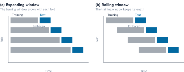
A backtest evaluates a forecaster on a sequence of forecast origins, each time training on the past of the origin and testing on the period that follows. It simulates the use of the forecaster in operation, and it gives a distribution of errors over periods instead of a single value [18], [22]. Figure 2.5 shows the two schemes. In an expanding window the training window keeps its start and grows by one test window at each fold, so the model is refitted on all the history. In a rolling window it keeps its length and moves, so the model forgets the oldest data. That is the better choice when the network changes or the record is costly to keep. In both, the training rows whose target lies in the test window are removed, which is the embargo of one horizon.
A single train-test split is the usual alternative, and it can name a winner that its own period happens to favour. Figure 2.6 scores the six forecasters on three single splits, each with one test window, and on the mean of the two backtests. The first split, January to April 2023, ranks the neural network first. The second, April to July 2023, ranks the previous day first and boosted trees fifth, which reverses the order of the learned families. The third, January to April 2024, ranks the neural network first again. Each of the three is a valid train-test split, and the conclusion of an operator who had computed only the second would be that no learned model beats yesterday. Both backtests give the same order: the neural network, boosted trees, the forest, ridge regression, the previous day and the previous week. The neural network scores 0.335 kW on the expanding window and 0.333 kW on the rolling one.
The backtests are also more informative than their means. The rolling window ranks the neural network first in four of the six windows, and the forest first in the last, where it is fourth. The ranking by window shows where a forecaster is fragile, and a recommendation that does not state it overstates what the evidence supports. The test windows should thus span every season of the year. A record without a winter would not show the benefit of the temperature, and a split that ends in one season reports the gain of that season only.
A split that assigns rows to folds at random breaks the order of time altogether, because the training rows then surround every test hour. The six forecasters are scored a second time on five random folds, on the same 12,553 test hours as before, so that only the way of splitting differs. The previous day and the previous week use no fitting, so they serve as a control whose error cannot change. Figure 2.7 gives the error of each forecaster on the expanding windows and on the random folds. On the random folds the learned families score lower, by 5% for ridge regression, 11% for the neural network, 14% for the forest and 15% for boosted trees. The more flexible the family, the larger the gain, because a flexible model can use the neighbours of a test hour that a random split places in its training rows. A ridge regression has few ways to do so. The gain is leakage, and a protocol that ignores time would report it as accuracy [20], [23], [24].
The ranking changes as well as the level. On the expanding windows the neural network is first in five of the six windows, and the previous day is first in April to July 2023 (Figure 2.8 (a)). On the random folds the previous day is fifth in every fold, boosted trees are first in four of five, and the neural network is first in one (Figure 2.8 (b)). A random split consequently reports that boosted trees are the best family and that no baseline can win, and both statements are false for the windows that follow the training.
Remark: the day as the unit of a test
The hours of one day share the weather and the habits of the households, so 24 hourly errors carry far less than 24 independent observations. Treating them as independent makes a small difference look significant. The daily mean of the loss is the unit that matches a day-ahead decision, and the number of days sets the power of the test.
Statistical Testing
A ranking by the mean error does not say whether a difference is reproducible or an accident of the days tested, and a hypothesis test answers that. The test of Diebold and Mariano compares the mean loss of two forecasters [25]. Let \(d_\tau = \mathcal{L}(e^{1}_\tau) - \mathcal{L}(e^{2}_\tau)\) be the difference between the daily losses of forecasters 1 and 2 on day \(\tau\). The null hypothesis is that its mean is zero, and the statistic is
\[ \mathrm{DM} = \frac{\bar d}{\sqrt{\hat\sigma^{2}_{\mathrm{HAC}} / n}}, \tag{2.24}\]
Here \(\hat\sigma^{2}_{\mathrm{HAC}}\) is a variance that allows for the serial correlation of \(d_\tau\). Under the null the statistic is approximately standard normal, so a large positive value says that forecaster 2 has the lower loss. The loss \(\mathcal{L}\) may be any score, so the test serves the absolute error, the squared error and the scores of probabilistic forecasts alike. The day is the unit, because the hours of one day are dependent. A forecast several steps ahead produces differences that are correlated over the horizon, so the variance allows for it with Bartlett weights [26],
\[ \hat\sigma^{2}_{\mathrm{HAC}} = \hat\gamma_0 + 2 \sum_{k=1}^{b-1} \Bigl(1 - \frac{k}{b}\Bigr) \hat\gamma_k, \tag{2.25}\]
where \(\hat\gamma_k\) is the autocovariance of \(d_\tau\) at lag \(k\) and the bandwidth \(b\) is seven days. The weights fall linearly to zero, which keeps the estimate positive.
The test of Giacomini and White asks a conditional question, whether one forecaster is better given what was known before the day [27]. It asks whether the difference is predictable from instruments \(\mathbf{h}_{\tau-1}\), here a constant and the difference of the previous day. With \(\mathbf{z}_\tau = \mathbf{h}_{\tau-1}\, d_\tau\) and the null that \(\mathbb{E}[\mathbf{z}_\tau] = \mathbf{0}\), the statistic is
\[ \mathrm{GW} = n\, \bar{\mathbf{z}}^{\top} \hat\Omega^{-1} \bar{\mathbf{z}} \;\sim\; \chi^2_q, \tag{2.26}\]
where \(\hat\Omega\) estimates the variance of \(\mathbf{z}_\tau\) and \(q\) is the number of instruments. It remains valid when the two models are fitted to the same data or one is nested in the other, which the test of Diebold and Mariano does not guarantee.
Both tests are pairwise, so six forecasters give \(C = 15\) comparisons. The Benjamini and Hochberg procedure orders the p-values \(p_{(1)} \le \dots \le p_{(C)}\) and rejects the hypotheses up to the largest \(k\) for which
\[ p_{(k)} \le \frac{k}{C}\, \alpha, \tag{2.27}\]
which bounds the expected share of false discoveries by \(\alpha\) [28]. With many forecasters a pairwise table is hard to read and may contradict itself. The model confidence set tests the hypothesis that all forecasters in a set have equal accuracy with the statistic
\[ T_{\max} = \max_{i} \frac{\lvert \bar d_{i} \rvert}{\sqrt{\widehat{\operatorname{Var}}(\bar d_{i})}}, \qquad \bar d_{i} = \frac{1}{M} \sum_{j} \bar d_{ij}, \tag{2.28}\]
Here \(\bar d_{ij}\) is the mean loss difference of forecasters \(i\) and \(j\), and \(M\) is the size of the set. The distribution of the statistic comes from a block bootstrap that respects the serial dependence. Whenever the hypothesis is rejected, the set drops the forecaster with the largest relative loss. It stops when no difference remains, and it returns the forecasters that cannot be separated from the best at a stated level [29]. The calibration of intervals is tested separately, and Chapter 3 treats it.
Figure 2.9 (a) applies the test of Diebold and Mariano to four pairs as the test sample grows from one window to six. The first named forecaster is expected to be better, and a small p-value means that it is. The neural network against boosted trees has a p-value of 0.24 on the 90 days of one window, which is no evidence. It is 0.014 on two windows and stays below 0.005 from 362 days on. A single window accordingly cannot separate two forecasters that differ by 2.5%, and several can. The reversal of the pair of boosted trees and ridge regression is a warning. On the first window the p-value is 0.003, which is significant at the 5% level, and on two windows it is 0.35. It returns to 0.023 on all six, so a conclusion drawn from the first window alone would have been reversed by the second. The neural network against the previous day falls from 0.10 on two windows to 1.5e-8 on all six. The fall comes mainly from the fifth window, where the gain of the neural network is largest.
The test of Giacomini and White rejects the equal conditional ability of every one of the four pairs, with p-values below 1e-6. It rejects even the pair of boosted trees and ridge regression, which the test of Diebold and Mariano leaves at 0.023. The difference between the two daily losses of that pair has a lag-one autocorrelation of 0.36. The advantage of one forecaster therefore persists from one day to the next and is concentrated in seasons. A mean difference does not show this, and it agrees with the ranks by window. The model confidence set points to the same conclusion from the other side. In the first window it keeps the neural network, boosted trees, the forest and the previous day, and in the second it keeps ridge regression as well. On the three windows from July 2023 to April 2024 it keeps two forecasters, and on all days it keeps the neural network alone.
Training Noise and Verdict
A network fitted twice with different seeds gives two different forecasts. A difference between forecasters that is smaller than that of two seeds of one forecaster is therefore not a difference. With \(S\) seeds, the noise floor is
\[ \delta = 1.96\, \frac{s}{\sqrt{S}}, \tag{2.29}\]
where \(s\) is the standard deviation over seeds of the mean absolute error. Under normality \(\delta\) is the half-width of a 95% interval for the mean over \(S\) seeds. For the neural network \(\delta\) is 0.0028 kW over three seeds. Boosted trees with fixed iterations have no randomness in their fit, and the floor of the forest is 0.0005 kW. Two forecasters are called equivalent when their errors differ by less than the larger of the floor and 1% of the error. That is the margin below which an operator would not act on the difference.
The verdict combines the evidence in one table (Table 2.2). The forecaster with the lowest error is the neural network. The other five all exceed it by more than the margin of 0.0034 kW. The adjusted p-values against it are below 0.011 for all five. The model confidence set at the 10% level holds the neural network alone. The protocol thus adopts the neural network, since the previous day errs 16.0% more. It also states that ridge regression is 5.8% above the neural network, which is significant, and that it is not separable from boosted trees or the forest. That is the reading that an operator needs, since it says what is known and where the evidence ends.
Table 2.3 lists the practices of the protocol, the failure that each prevents and where the chapter shows that failure.
| Practice | Failure that it prevents | Shown in |
|---|---|---|
| Report the skill against the previous day | A weak baseline makes a model look better than it is | Comparison on One Transformer |
| Choose the score from the decision | The ranking answers a different question | Evaluating a Point Forecast |
| Report the error by hour | A good average hides a failure in the hours that matter | Evaluating a Point Forecast |
| Split in time, with an embargo of one horizon | Leakage lowers the error of flexible models by 5% to 15% | Protocol for Comparing Forecasters |
| Use windows of every season | One season names a winner that the others reverse | Protocol for Comparing Forecasters |
| Test on daily losses, adjusted for the pairs | Dependent hours and many pairs make a difference look real | Protocol for Comparing Forecasters |
| State the noise floor and the equivalence margin | A difference smaller than the noise of training is reported | Protocol for Comparing Forecasters |
The findings are those of one transformer of 18 customers over 33 months. They use one set of inputs, an observed weather that stands for a perfect forecast, and models with fixed settings. A tuned model, a longer record or a forecast weather would move the numbers. The methods of the protocol do not depend on those choices, and they are the part that transfers. They are a split in time, a baseline, a paired test on daily losses, a noise floor and a ranking by window.
Pitfall: a random split on a time series
A random split lets the training rows surround every test hour. The error then falls by 5% to 15% for models that can interpolate, and the ranking shows a winner that the later days do not confirm. Split in time, with an embargo, and include every season.
Benefit of Input Sets
Chapter 1 ranked the inputs by their relevance, and a ranking only shortlists them. This section applies the protocol above to a question that a ranking cannot answer. The question is whether an input set lowers the error of a forecaster that already has the calendar. It is measured on the Porsgrunn transformer and on series of known truth.
Benefit on Expanding Windows
The benefit of an input set is measured on expanding windows [22], [23], [30]. The first model is trained on 12 months and tested on the next three. The training window then grows by those three months and the test window moves on, so that no model sees the future of its test window. Training rows whose target lies in the test window are dropped, because a forecast issued on the last day before the window has its outcome inside it. The record gives six test windows of about 2,100 hours each, from January 2023 to June 2024. They cover every season and the winter twice. Every set is fitted with the same boosted-tree regression [8], with a fixed number of iterations, on the same windows, so the sets differ only in their inputs. The forecast is direct at 24 hours ahead, with the calendar and the weather of the target hour as inputs. The error is the mean absolute error \(\mathrm{MAE}_S = n^{-1}\sum_t \lvert y_t - \hat{y}_t^{(S)} \rvert\) in kW per customer. The benefit of a set \(S\) over the calendar alone is the skill [31]
\[ \mathrm{skill}_S = 1 - \frac{\mathrm{MAE}_S}{\mathrm{MAE}_{\mathrm{cal}}}. \]
It is the share of the error of the calendar that the added inputs remove, and it is negative when they add error.
Remark: the weather of the target hour
The benefit is measured with the observed weather of the target hour, as if the forecast of the weather were perfect. An operator receives a forecast with its own error, so the benefits below are upper bounds, and the final choice should be tested on archived forecasts. The order of the inputs can change when the forecast error of one variable exceeds that of another.
Known Truth and Transformer
The known truth shows what the error against the outcomes hides. The outcomes carry noise that no input can remove, so the error against them changes little. The mean absolute error is 1.577 kW for the calendar and 1.478 kW with the irradiance, a fall of 6%. The distance of the forecast from the true conditional mean, which exists only for the synthetic series, falls from 0.840 kW to 0.449 kW, a fall of 47% (Figure 2.10). The temperature alone gives 0.888 kW, worse than the calendar, and added to the irradiance it raises the distance from 0.449 kW to 0.491 kW. The load of the previous day gives 0.905 kW and the noise 0.880 kW. These three sets exceed the calendar by 0.04 to 0.07 kW, at least three standard deviations of the three seeds, so the differences are reproduced and not random. The load of the previous day and the temperature rank third and fifth in Figure 1.22. They carry no benefit over the calendar, which already holds the season and the daily cycle. A model pays for an input of no value in variance. The benefit must therefore be tested for every input that a ranking proposes, since the ranking alone cannot show that an input adds nothing.
On the Porsgrunn transformer the mean absolute error of the calendar alone is 0.461 kW per customer. The temperature reduces it to 0.344 kW, a skill of 25.3% (Figure 2.11). One temperature forecast added to the calendar therefore removes about a quarter of the error of the day-ahead forecast, the largest benefit of the single inputs tested. All ten weather variables together give 0.353 kW (23.6%), the feels-like temperature 21.8%, the load 24 hours earlier 17.7%, the dew point 9.0% and the solar radiation 2.9%. The column of noise (−0.9%) and the pressure (−5.6%) add error. With the temperature the root mean squared error falls from 0.586 kW to 0.432 kW, a fall of 26%. The large errors thus fall as well as the typical ones. The bias of the calendar is 0.088 kW of under-forecast on average, and it falls to 0.022 kW. A forecast that under-forecasts on average understates the loading of the transformer, so the removal of the bias matters to the operator as well as the fall of the error. The fusion is right at the top and at the bottom, since the temperature is among the first and the noise among the last. It is not right in the middle: the pressure ranks sixth and loses 5.6%, while the dew point ranks fifth and gains 9.0%. A ranking can consequently shortlist the inputs but cannot replace the backtest.
The benefit depends on the season, which a single average would hide. The temperature removes 41.5% of the error in October to December 2023 and 38.8% in January to March 2024. In July to September 2023 it removes 0.4%, when the calendar alone has its lowest error of 0.304 kW. The calendar errs most in the cold windows, with 0.652 kW and 0.529 kW, because the cold of one winter is not in the calendar and the temperature supplies it. The temperature gains in every window, by at least 0.4%, whereas the noise loses in all six and the pressure in five. A single split that ends in one season would report the gain of that season only. A record without a winter would not show the benefit of the temperature at all.
The differences are tested with the paired test of Protocol for Comparing Forecasters on the daily mean absolute errors of the 545 test days. The bandwidth is seven days, and the p-values are adjusted over the 36 pairs of the nine sets. Figure 2.12 gives the size of the reduction for every pair, and each pair that does not differ significantly prints its adjusted p-value. Of the 36 pairs, 35 are significant, so the test alone does not separate the sets. Even the calendar and the calendar with noise differ significantly, by 0.004 kW or 0.9% of the error, which no operator would act on. The skill says whether a difference matters and the test whether it is reproducible, and both are reported. The temperature alone outperforms all ten weather variables together with an adjusted p-value of 0.0498, slightly below the level, and it outperforms the feels-like temperature, with 0.007. The ten variables together and the feels-like temperature cannot be told apart, with 0.081. The other nine variables accordingly do not help a model that already has the temperature, and the evidence that they harm it is weak.
The findings are those of one transformer, one family of models with a fixed number of iterations, six test windows, and an observed weather that stands for a perfect forecast. The known-truth series are a single Gaussian factor with PV. A network without electric heating, such as a PV-rich feeder, ranks the irradiance first, as the synthetic series do. Two PV-rich LV substations behaved alike: the irradiance carried the benefit, and the temperature added nothing to it [15]. The choice of inputs therefore has to be repeated for each network.
The simplest adequate set is the calendar with the temperature. It gives a skill of 25.3% against 23.6% for all ten weather variables, it needs one weather forecast and not ten, and it gains in every window. To select the inputs of a new forecaster, take the shortlist of Chapter 1 and follow these steps.
- Fit the sets that the shortlist proposes, and the calendar alone as the reference, on expanding windows that include every season.
- Read the skill of each set in each window, and test the daily errors in pairs with the adjustment for the number of pairs.
- Keep the smallest set whose skill is within the noise of the best, and report the skill by window next to the test.
The calendar with the temperature is the input set that the comparison of Comparison on One Transformer holds fixed for the Porsgrunn transformer. The irradiance is the input for a PV-rich net load.
Comparison on One Transformer
The six forecasters are fitted on the expanding windows of Protocol for Comparing Forecasters, with a first window of 12 months and test windows of three months. The training rows whose target falls in a test window are removed. The settings are fixed and not tuned, so that no family has had more effort than another. The learned families read the calendar and the temperature of the target hour. The error is the mean absolute error, and the skill is its reduction against the previous day, which is the reference of the operator. Figure 2.13 gives the skill in each window.
All four learned families beat the previous day on average. The neural network does so by the most, with a skill of 13.8%, which is an error of 0.335 kW per customer against 0.389 kW. Boosted trees give 11.7%, the random forest 10.7% and ridge regression 8.8%. The previous week is 26.0% worse than the previous day, since a week-old load carries the weekday and the weather of another week. The gain depends on the season, and in January to April 2024 the neural network removes 31.1% of the error of the previous day. This is consistent with changes of temperature between days that a repeated load cannot see. In April to July 2023 the neural network is 0.5% worse than the previous day, and boosted trees and the forest are 5.5% worse. The load of the previous day is then as good as any model, which appears to be because the temperature has little to explain in spring. A model judged on that window alone would not justify its fitting, and a model judged on the winter alone would be overrated.
Figure 2.14 shows two situations on one week each. In the winter week the load falls towards the weekend, which the previous day cannot know, since it repeats a weekday on a Saturday. The neural network follows the fall, with a mean absolute error of 0.334 kW against 0.538 kW. In the spring week the neural network forecasts the weekdays too high, with 0.529 kW against 0.314 kW for the previous day. The weeks are chosen to show the two situations and are not typical. They show what an average hides, since a forecaster that is better on average can miss a whole week. A plot of this kind only checks that the cycle is followed, because the eye reads the horizontal distance between curves and the error is the vertical one [18]. The daily errors beneath each week carry the comparison.
The differences among the learned families are small against their difference from the baselines. The neural network has a mean of 0.338 kW over three seeds, with a standard deviation of 0.002 kW. Its lead of 0.006 kW over boosted trees is consequently more than twice the variation between runs. The paired test on the daily errors of the 544 test days, with the bandwidth and the correction of Protocol for Comparing Forecasters, finds 13 of the 15 pairs significant (Figure 2.15). The neural network is better than the other three learned families, by 2.5% against boosted trees, 3.6% against the forest and 5.6% against ridge regression. Ridge regression cannot be told apart from boosted trees, with an adjusted p-value of 0.0502, or from the forest, with 0.195.
The cost decides among the families that the test cannot separate. One fit on the 18,791 training rows of the last window takes under 0.01 s for ridge regression and 0.45 s for the forest. It takes 1.06 s for boosted trees and 2.41 s for the neural network, which also needs scaled inputs and a seed that is fixed and checked. Ridge regression gives 8.8% of the 13.8% of the best family, at no fitting cost and with weights that an engineer can read. It is accordingly adequate on average for this transformer. The neural network is justified only where a further 5.6% of the daily error repays the maintenance of a monitored model. An average over the day can still hide a failure, and the next section shows that ridge regression has one in the morning.
Pitfall: a model compared with a weaker baseline
A learned model that is compared only with the previous week, or with no baseline, looks far better than it is. The previous day is the reference of an operator. Report the skill against it, window by window, and state the windows in which it wins.
Scores Compared
Figure 2.16 reads the six forecasters under nine measures, each cell printing the value and shading its excess over the best. The mean and the median absolute error, the root mean squared error, both scaled errors and the normalised error order the six identically. The neural network is first and the previous week last. The percentage error swaps the forest and ridge regression, ranking ridge third and the forest fourth, and the symmetric percentage error keeps the order of the absolute error. The scaled error is 0.998 for the neural network, so it is as accurate on the test windows as the previous day was in the first year of the record. The previous day itself scores 1.158, so it errs 16% more on the test windows than in the first year, which no unscaled error shows.
The median absolute error of the neural network is 0.282 kW against a mean of 0.335 kW. The ratio of the two lies between 0.81 and 0.85 for every forecaster. The tails of the errors are alike, so the ranking does not rest on a few large misses. The margin for a critical event is set at 20% of the mean load of the training period, which is 0.475 kW per customer. The neural network exceeds it in 25.4% of the hours and the previous day in 31.8%, so the neural network removes a fifth of the hours with a large miss. The mean error is within 0.04 kW for every forecaster, which is below 8% of the mean absolute error for the previous week and smaller for the others. No forecaster leans enough to bias a reserve. The normalised bias is negative for all six forecasters, between -0.018 and -0.001, whereas the mean error of boosted trees, the forest and ridge regression is positive. The two readings differ because the normalised bias weights every hour alike and so follows the low loads, and the mean error follows the large loads. These three families therefore forecast too high at low load and too low at high load.
The percentage error also changes which period looks hardest. Figure 2.17 ranks the six test windows of the neural network under the two errors. The window of October to December 2023 is the hardest in kW, with rank six. It is the second easiest in percent, because the winter load is large and turns the same error into a small percentage. A forecaster judged by the percentage error would be thought most reliable in the season where it errs most in kW.
Error by Hour
A single number over the whole day weights every hour alike, whereas the decisions of an operator do not. The evening peak sets the loading of the transformer, and the ramp of the morning sets the reserve that must be ready. Figure 2.18 gives the error of three forecasters by the hour of the target.
At the evening peak, hours 19 to 21, the neural network and ridge regression have almost the same error, 0.360 kW and 0.364 kW. The previous day errs by 0.435 kW, which is 21% more than the neural network. In the morning ramp, hours 6 to 8, the order changes. The previous day has an error of 0.304 kW and the neural network 0.302 kW, whereas ridge regression has 0.359 kW, which is 18% more than the previous day. A linear model on the sine and cosine of the hour appears unable to follow a load that rises at a fixed time of the morning and then falls. The family that was adequate on average is therefore not adequate for the decision that the morning serves. Its average of 0.355 kW hides a failure of 18% in the hours that set the morning reserve, which only an error by hour shows.
Further Applications
A forecaster that has been compared on one transformer is useful only if the comparison carries to the problems that an operator meets next. Each of them changes one choice, the quantity, the horizon or the information set, while the protocol stays the same.
The first is a meter without history, for which no model can be fitted. The previous day and the previous week serve from the first week, and a seasonal profile from the first year. The retrieval of similar customers supplies a forecast from the meters that resemble it. A second is the forecast of the charging of electric vehicles, where the share of the error in the largest steps (Evaluating a Point Forecast) shows what an average hides. The two apply the baselines and the skill of this chapter without a change.
A third is the voltage at the end of a feeder, which has been forecast jointly with the active and the reactive power [32]. The target is a bounded quantity with a regulatory band, so a point forecast scored by the squared error misses the quantity that matters, the exceedance of the band. Chapter 3 forecasts the distribution of such a quantity, and the protocol of Protocol for Comparing Forecasters applies unchanged. The same holds for a decision with asymmetric costs, such as the purchase of energy or the sizing of a reserve, where the costs set the quantile that is needed.
In each application the questions are the same. They are what the information set contains at the origin, what the decision needs from the forecast, and which baseline the forecaster has to beat in every season. The methods that follow in this part change the form of the forecast and not the discipline of its evaluation.
Conclusion
The chapter followed one question, which forecaster to run and how to know that it is better than another, from the family of models to the verdict of a test. The families of models were compared with the inputs held fixed (Comparison on One Transformer), and the neural network led with a skill of 13.8% against the previous day. Ridge regression held 8.8% at no fitting cost, but it failed in the morning ramp, and the previous day won in the window of spring (Model Families). The evaluation showed that the squared and the absolute loss target the mean and the median, and that the percentage error flatters a low forecast. It also showed that an error by hour exposes a failure that the average hides (Evaluating a Point Forecast). A random split lowered the error of flexible models by up to 15% and changed their order. A single split named the previous day as the winner in one of three periods. The test sample had to span several windows before two forecasters could be separated (Protocol for Comparing Forecasters). The test of benefit showed that the calendar with the temperature was the simplest adequate set, and that the rank of an input did not predict its benefit (Benefit of Input Sets).
Scope and limitations
The findings come from one transformer of 18 customers over 33 months, an observed weather used as a perfect forecast, models with fixed settings, and synthetic series of one structure. They fix the method of evaluation, and the numbers have to be remeasured for another network.
Table 2.4 sets out the choices that an operator makes, by the information that is available. The table reads from left to right: the baseline to beat, the family to try first, the score to report and the check before use. The rows follow the findings of this chapter and are a starting point to be tested on the neural network at hand.
| Context | Baseline | Family to try first | Score | Check before use |
|---|---|---|---|---|
| A year or more of hourly load and a temperature forecast | Previous day and previous week | Ridge regression on the calendar and the temperature | Absolute error and skill against the previous day | Expanding windows of every season, the error by hour and the daily test |
| Two years of load and a rich weather forecast | Previous day | Boosted trees or a small neural network, after ridge regression | Absolute error beside the root mean squared error | The ranking by window, the seeds and the cost of fitting |
| A net load with PV that crosses zero | Previous day | The irradiance as the first input, then the calendar | Absolute error, never the percentage error | The season of the cloudy days, and the skill by hour |
| A household or a small feeder | Previous day | The calendar only, with the previous day as the fallback | Absolute error against the daily naive error | The forecastability of the series, which may leave nothing to gain |
| Less than a year of load | Previous week | None learned | Absolute error | Collect a full year before fitting |
| A forecast of the next hours, refreshed as the meter reports | The last observed value | Ridge regression on the latest lags and the calendar | Absolute error by lead time | Skill against the last value at each lead time, because lags shorter than a day become admissible |
| A decision with asymmetric cost | Previous day | A quantile forecast | The pinball loss at the needed level | Coverage by window (Chapter 3) |
The trade-offs of the table carry numbers, and the gain of a flexible family has a cost. A neural network gains 5.6% of the daily error over ridge regression and costs 2.41 s to fit against under 0.01 s. It pays only where the maintenance of a monitored model is repaid. A random split lowers the error by up to 15% for a flexible family and reports a ranking that the later days do not confirm. A percentage error shifts the ranking of two families by one place on a positive load, and it would shift it by more on a net load. The chapters that follow turn from the point forecast to the distribution of the load, and from the load to the neural network quantities that it drives.
Exercises
- A utility holds hourly load and a temperature forecast for 40 transformers of 20 to 60 customers. It asks which family of model to run day-ahead on all of them. Design the comparison by stating the baseline, the windows, the test, the score, the margin of equivalence and the check that the result transfers to a new transformer. State what to report if ridge regression and boosted trees cannot be separated.
- Let the outcome \(y\) have a lognormal distribution with parameters \(\mu\) and \(\sigma\). Show that its mean exceeds its median and derive the ratio of the two. Show that the median has the lower expected absolute error and the mean the lower expected squared error. Relate the ratio to the gap of 0.69 kW found for the lognormal series of Evaluating a Point Forecast.
- Show that the seasonal naive forecast of Equation 2.3 with \(m = 24\) and \(h = 24\) repeats the load of the origin hour. Show that a lag shorter than the horizon would lie after the origin. In the companion notebook, shorten the lag of one input set to 12 hours and measure the apparent gain on the expanding windows.
- Derive the variance of the mean of \(n\) dependent daily loss differences with autocovariances \(\gamma_0, \gamma_1, \dots\) up to lag \(q\). Show how the Bartlett weights keep the estimate positive.
The Chronos models are an example, with code at https://github.com/amazon-science/chronos-forecasting.↩︎