Non-Intrusive Load Monitoring
In 2016, a team at the University of Virginia asked a strange question: could you guess which appliances a household owns from nothing but its monthly electricity bill? One number, thirty days apart. No smart meter, no sub-metering, just the figure already printed on every utility invoice. Their system, Gemello, could still flag a house as likely owning a space heater or an old refrigerator, just from the shape of that one number over time [1].
That is Non-Intrusive Load Monitoring (NILM) taken to its extreme: almost no signal, and still something real to say about what is running behind the meter. Most of this book works with a much richer signal than a monthly bill, readings every few seconds or minutes, but the underlying problem is the same one Gemello solves in miniature. Given only the aggregate power drawn at a single point, can you recover what individual appliances are doing?
Key Concept
Formally, a smart meter reports one aggregate signal \(x_t\) at each time step \(t\). Behind it, \(M\) appliances are each drawing some power. NILM recovers, for every appliance \(k\), both its on/off state \(s^{(k)}_t\) and its power draw \(y^{(k)}_t\), such that
\[ x_t = \sum_{k=1}^{M} y^{(k)}_t \cdot s^{(k)}_t + \sigma_t \]
where \(\sigma_t\) absorbs measurement noise and anything not accounted for. Nobody observes \(y^{(k)}_t\) or \(s^{(k)}_t\) directly. Recovering them from \(x_t\) alone is the entire problem [2].
Run the cell below and the problem stops being abstract. It builds one day of a synthetic household: a roughly constant baseline load from lights and standby devices, a fridge cycling on and off every half hour or so, and a kettle spiking twice a day. The aggregate line at the top is all a real smart meter would ever report. The other three are exactly what disaggregation has to recover, and they are already invisible once summed.
Notice how the fridge and the baseline load barely show up once the kettle’s spike is on the same axis. That is not a plotting choice, it is the actual shape of the problem: a smart meter’s one number is dominated by whatever draws the most power at that instant, and the rest has to be inferred, not read off.
High frequency or low frequency: two different jobs
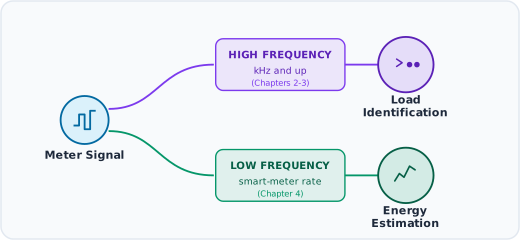
Before any of the four steps run, one choice already shapes everything that follows: how fast is the meter actually sampling? The literature splits roughly into two regimes, and each one is suited to a different question [3].
High-frequency acquisition, kilohertz and up, captures the transient noise an appliance’s switch-mode power supply puts back onto the line: shape, harmonics, the brief spike before a device settles into steady state. That detail is what makes it possible to tell a kettle from a hair dryer even when both draw similar average power. Patel and colleagues built custom hardware to capture exactly this, sampling the range to fingerprint individual switching events on the residential power line [4]. The cost is real: that hardware does not exist in a standard smart meter, so high-frequency NILM is fundamentally a load identification problem, telling appliances apart, answered with equipment most households do not have.
Low-frequency acquisition, on the order of one reading every few seconds to a few minutes, is what an actual deployed smart meter reports. There is no transient detail to lean on here, so the question changes: not “which exact appliance is this” but “how much energy is being used, and by roughly which category of load.”
Both regimes matter to this part of the book, and for a specific reason: high-frequency, event-level measurement is where the author’s own published research sits (Chapters 2 and 3), while low-frequency, smart-meter-rate data is where the field’s modern deep-learning tooling operates at scale (Chapter 4). Figure 4.1 lays out that fork.
Detecting when something changed
A NILM system has to detect an appliance’s operating status, ON or OFF, or a finite state somewhere between the two, from the power measurements alone. This is harder than it sounds: appliances differ widely in the statuses they can be in, from simple ON/OFF, to a finite set of states, to always-ON, to continuously variable [2]. Based on how they approach this, NILM methods split into two families: event-based and state-based (also called non-event-based).
Event-based approaches focus on the state-transition edges an appliance generates and use a change-detection algorithm to identify where an event starts and ends [5], [6]. The job of the change-detection algorithm is to spot changes in the aggregate load time series caused by one or more appliances switching ON/OFF or changing state. This relies on the fact that power monitored in a home is continuously rising, falling, and stepping. When a change is significant enough, it is taken as evidence that an event occurred. Appliance signatures, such as active power or the size of the rising or falling edge, are then analyzed to classify which event it was. A review of event-detection algorithms used in the NILM literature is given in [7]. The performance of event-based approaches is limited by the fixed or adaptive threshold of the change-detection algorithm, by measurement noise, and by similarities among steady-state signatures; missed detections and false detections of edges are both common failure modes.
State-based approaches do not rely on an event detector at all. Instead they rely on pattern recognition: an appliance turning ON/OFF or changing running state creates a distinct pattern with a probability distribution that matches that appliance. At low sampling rates, the classic example is the Hidden Markov Model [8], [9], though it is not a method this book spends much time on: modern deep-learning approaches have largely taken its place for low-frequency energy estimation, and Chapter 4 picks up that thread directly.
Event-based methods tend to pair naturally with the high-frequency, load-identification problem above; state-based methods are the more common choice once the signal is low-frequency and the goal shifts toward energy estimation.
Telling appliances apart
An effective NILM algorithm needs signatures unique enough to characterize appliance behavior: a distinctive energy-consumption pattern, often called its appliance signature, that identifies and recognizes that appliance’s operation from the aggregate load. Hart frames it the same way: a measured parameter of the total load that carries information about one appliance’s nature or operating state, a consumption pattern intrinsic to that device [2], [3], [10]. NILM research uses two main classes of signature: transient and steady-state.
Transient signatures are short-term fluctuations in power or current before the appliance settles into a steady-state value. They uniquely define appliance-state transitions through features like shape, size, duration, and harmonic content of the transient [3]. Capturing them requires high sampling rates, to get a high degree of signal uniqueness, and longer monitoring time, to capture a full operating cycle, which in turn demands hardware more costly than the low-frequency power a smart meter reports. Patel and colleagues, for example, built custom hardware to detect transient noise across , exploiting the fact that an appliance’s in-state operation transmits noise back onto the power line [4].
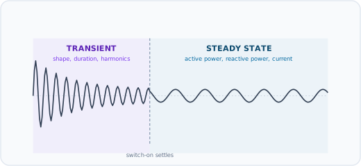
Steady-state signatures relate to the more sustained change in power characteristics once an appliance settles into a running state. At the low-frequency end, these include active power [10], [11], reactive power [12], and current [13], the signatures a smart meter can actually supply, which is why they dominate the practical low-frequency NILM literature. Where most prior work uses real power for NILM [9], [11], [14], Makonin and colleagues argue that current, rather than real power, is the more effective steady-state feature for energy disaggregation [13], a useful reminder that the obvious choice of feature is not always the best one.
The Voltage-Current (V-I) trajectory, the closed loop traced by plotting instantaneous voltage against instantaneous current over one cycle, is also technically a steady-state signature, but it belongs to the high-frequency side of the split above: tracing a stable, recognizable loop shape needs sampling in the tens of kilohertz, not the sub-hertz rate a smart meter reports [15]. This distinction matters more than it might seem. Chapters 2 and 3 of this part both build on the high-frequency, event-based, load-identification side of NILM: turning that V-I loop, or the raw activation current itself, into an image-like or graph-like representation a classifier can learn from [15], [16].
From features to an answer
Once a signature has been extracted, it can be used to identify the appliance category, its status, and its power consumption. Machine learning models do this in two stages: a learning stage that fits model parameters, and an inference stage that infers appliance states from observed aggregate power and estimates their power consumption.
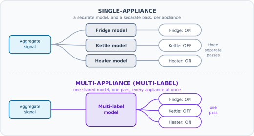
Single-appliance or multi-appliance. NILM learning strategies further split into single-appliance learning, which assumes only one appliance is active at a time and disaggregates one appliance at a time, and multi-appliance learning, which links several appliances to one observed aggregate signal at once [17]. Single-appliance learning ignores the fact that appliances can be active simultaneously and that their usage is not independent, yet it is the strategy behind most deep-learning NILM models, each trained on one particular appliance. Multi-appliance, multi-label learning is the more realistic setting and the one Chapter 3 of this part deals with directly.
Power estimation. Historically, low-frequency energy estimation leaned heavily on HMM variants, including the factorial HMM, an extension that tracks several appliances’ hidden states jointly rather than one at a time [18]. This book does not spend much time there either: Chapter 4 covers how modern deep learning handles power estimation at low frequency instead.
Why bother
The case for disaggregation is not really about the appliance breakdown itself. It is about what that breakdown lets someone do next. A household that can see its fridge is drawing twice what a healthy fridge should, before the fridge fails outright, gets to fix it on their own schedule instead of throwing out a freezer full of food [19], [20]. A retailer that can separate heating load from everything else can price and forecast far more precisely than one working from a single aggregate curve. None of that requires solving NILM perfectly, it requires solving it well enough to be useful, which is a lower and more interesting bar, and one Barker and colleagues argue the field should judge itself by explicitly, instead of chasing accuracy numbers on a benchmark no household ever sees [21], [22].
That bar shows up in a handful of recurring, real use cases, well beyond splitting a single bill into a per-appliance breakdown:
- Actionable feedback. A number is not the same thing as a decision. Batra and colleagues found that showing a household its heating, its fridge, and its lighting as separate lines, not one combined total, is what actually changes behavior, because a person can only act on a category they can see [23].
- Fault detection. The fridge example above is not hypothetical. A fridge’s compressor draws a distinctive, repeating cycle; once NILM can isolate that cycle, a lengthening cycle time or a rising baseline draw is an early warning sign a technician can act on before the unit fails [19], [20], [24].
- Continuous energy audits. A manual walk-through audit is a snapshot: an auditor visits once and inspects what is running that day. Berges and colleagues showed NILM output can stand in for, or extend, that audit continuously, catching an oversized or aging piece of equipment without scheduling a site visit [25].
- Demand response. A utility that already knows how much of a home’s load is heating, cooling, or one specific flexible appliance can target a demand-response signal at exactly that slice of load, instead of asking a household to guess what to turn off during a peak event [26], [27].
- Occupancy and household characteristics. Because NILM output already reflects which appliances are running and when, the same signal can be read backward: an empty house looks different from an occupied one, and an unsupervised model built entirely from unlabeled smart-meter data, with no household ever filling out a survey, can pick that up directly [28].
None of this is speculative. Sense and Bidgely are two commercial products built on exactly this idea, disaggregating a home’s smart-meter or panel-level signal into appliance-level insight and selling the result back to the household or the utility.
Datasets exist precisely so this problem can be studied properly: real households or industrial sites, metered at the aggregate level and, critically, with ground-truth sub-meters on individual appliances to check any disaggregation algorithm’s answers against. Low-frequency datasets like UK-DALE support the energy-estimation side of NILM [29]; high-frequency, event-level datasets support the load-identification side. Later chapters in this part use both, depending on which problem is on the table.
Where this part of the book goes
This chapter only frames the problem. The rest of Part 2 builds the actual methods, following the high-frequency/low-frequency split this chapter introduced:
- Chapter 2, feature engineering for appliance recognition, moving into the high-frequency, event-based side of NILM: turning the V-I trajectory or activation current into a graph-based representation that makes appliances easier to tell apart, then extending that same representation to three-phase industrial settings, where phase imbalance becomes a challenge, and an opportunity, of its own.
- Chapter 3, multi-appliance recognition, extending that same high-frequency representation to the more realistic case where several appliances change state at once, not one at a time.
- Chapter 4, deep learning at low frequency, back on the energy-estimation side: modern neural architectures benchmarked reproducibly on UK-DALE, where a model learns its own features directly from the aggregate signal.
Common Mistake
Assuming NILM always needs labeled, sub-metered training data. Some methods do. Others, including several covered later in this part, work from the aggregate signal alone. Which one is appropriate depends entirely on what data is actually available at deployment time, not on which method has the best published accuracy.