


Beyond energy: hourly web traffic#
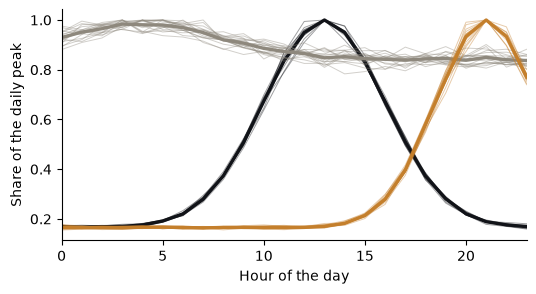
Nothing in milia is specific to electricity. This tutorial clusters the hourly traffic of forty pages and flags a day on which one page went down, with the same functions as the load-profile tutorials. The data are synthetic.
import matplotlib.pyplot as plt
import numpy as np

from milia import make
from milia.anomaly.ensemble import Ensemble
from milia.cluster import selection, validation
from milia.features.window import vector

BLACK, GREY, OCHRE = "#111318", "#8E887D", "#C47F2C"
rng = np.random.default_rng(7)
hours = np.arange(24)
bump = lambda centre, width: np.exp(-0.5 * ((hours - centre) / width) ** 2)  # noqa: E731

# Three kinds of page: read in office hours, read in the evening, and crawled evenly around the clock.
patterns = {"Office hours": 0.2 + bump(13, 3), "Evening": 0.2 + bump(21, 2.5), "Crawlers": 0.6 + 0.1 * bump(4, 4)}
kinds = rng.integers(0, 3, size=40)
base = np.array(list(patterns.values()))[kinds]
days = base[:, None, :] * rng.lognormal(0, 0.15, size=(40, 60, 24))  # pages by days by hours
days.shape
(40, 60, 24)
Cluster the pages by the shape of their day#
shapes = days.mean(axis=1)
shapes = shapes / shapes.max(axis=1, keepdims=True)
scores = validation.sweep(shapes, range(2, 7), resampling=True)
k = selection.recommend(scores, strategy="trust")
labels = make("clusterer", "kmeans", n_clusters=k, random_state=0).fit_predict(shapes)
k, validation.external(labels, kinds)
(3, {'ari': 1.0, 'nmi': 1.0000000000000002, 'purity': 1.0})
fig, ax = plt.subplots(figsize=(6, 3))
for c, colour in zip(range(k), (BLACK, GREY, OCHRE), strict=False):
    ax.plot(hours, shapes[labels == c].T, color=colour, lw=0.7, alpha=0.4)
    ax.plot(hours, shapes[labels == c].mean(axis=0), color=colour, lw=2.4)
ax.set(xlabel="Hour of the day", ylabel="Share of the daily peak", xlim=(0, 23))
ax.spines[["top", "right"]].set_visible(False)
plt.show()
Flag the day a page went down#
One page loses most of its traffic on day 45. The detector is fitted on that page’s normal days.
page = 3
series = days[page].copy()
series[45] *= 0.1  # an outage
features = [vector(day) for day in series]
normal = [i for i in range(60) if i != 45]
detector = Ensemble().fit([features[i] for i in normal[:40]])
detector.calibrate([features[i] for i in normal[40:]], alpha=0.1)
np.flatnonzero(np.asarray(detector.flag(features)))
array([13, 45, 51])
The same four steps, features, fit on normal data, calibrate on held-out normal data, flag, applied to a quantity with a different rhythm and a different unit. The synthetic outage is easier than a real one, so treat the result as a check that the pipeline runs, not as a benchmark.