Quickstart

This page builds a small low-voltage network, solves it, checks its voltages against a standard and simulates one day with rooftop solar. Every output on the page is produced by the code above it when the documentation is built. To run it yourself, install the opendss and plot extras (see Installation).

Build a network

A Circuit attaches to the OpenDSS engine. You define the network with OpenDSS’s own commands: here an 11/0.4 kV transformer, a 1 km cable and three houses, one on each phase.

from popo.network import Circuit

circuit = Circuit()
for command in [
    "Clear",
    "Set DefaultBaseFrequency=50",
    "New Circuit.Quickstart",
    "Edit Vsource.Source bus1=SourceBus basekv=11 pu=1.0 phases=3",
    "New Transformer.LVTR Buses=[SourceBus, A.1.2.3] Conns=[delta wye] KVs=[11, 0.4] KVAs=[250 250] xhl=2.5",
    "New Linecode.240sq nphases=3 R1=0.127 X1=0.072 units=km",
    "New Linecode.16sq nphases=1 R1=1.15 X1=0.083 units=km",
    "New Line.A_B bus1=A.1.2.3 bus2=B.1.2.3 length=1 units=km linecode=240sq",
    "New Line.B_C bus1=B.1 bus2=C.1 length=0.02 units=km linecode=16sq",
    "New Line.B_D bus1=B.2 bus2=D.2 length=0.02 units=km linecode=16sq",
    "New Line.B_E bus1=B.3 bus2=E.3 length=0.02 units=km linecode=16sq",
    "New Load.House_C bus1=C.1 phases=1 kV=0.23 kW=7 pf=0.95",
    "New Load.House_D bus1=D.2 phases=1 kV=0.23 kW=6 pf=0.95",
    "New Load.House_E bus1=E.3 phases=1 kV=0.23 kW=8 pf=0.95",
    "Set VoltageBases=[11 0.4]",
    "CalcVoltageBases",
]:
    circuit.command(command)
circuit.solve()
circuit.converged

True

Inspect its elements

The circuit yields its lines, loads, transformers, PV systems and storage units as records, which convert directly to a DataFrame.

pd.DataFrame(circuit.loads)

	name	bus1	kw	kvar	pf	phases
0	house_c	c.1	7.0	2.301	0.95	1
1	house_d	d.2	6.0	1.972	0.95	1
2	house_e	e.3	8.0	2.629	0.95	1

Read the results

bus_voltages() returns one row per bus and connected phase. House D appears only on phase 2 and house E only on phase 3, the phases they are connected to.

voltages = circuit.bus_voltages()
voltages

	bus	phase	vmag_pu	vangle_deg	kv_base
0	sourcebus	1	1.000	-4.915e-04	6.351
1	sourcebus	2	1.000	-1.200e+02	6.351
2	sourcebus	3	1.000	1.200e+02	6.351
3	a	1	0.999	-3.012e+01	0.231
4	a	2	0.999	-1.501e+02	0.231
5	a	3	0.999	8.987e+01	0.231
6	b	1	0.982	-3.046e+01	0.231
7	b	2	0.982	-1.501e+02	0.231
8	b	3	0.972	8.947e+01	0.231
9	c	1	0.979	-3.041e+01	0.231
10	d	2	0.979	-1.500e+02	0.231
11	e	3	0.968	8.952e+01	0.231

summary() gives the size of the circuit, whether it converged and its total losses.

circuit.summary()

{'converged': True,
 'n_buses': 6,
 'n_lines': 4,
 'n_loads': 3,
 'n_transformers': 1,
 'total_p_loss_kw': 0.49856510379089014,
 'total_q_loss_kvar': 0.30006894118455557}

Check against a standard

VoltageLimits holds a standard’s band and the rule for applying it. The source bus is held at its setpoint, so it is excluded before the check.

from popo.standards import VoltageLimits

limits = VoltageLimits.en_50160()
customers = voltages.query("bus != @circuit.source_bus")
print(limits.check(customers["vmag_pu"]).summary())

EN 50160: compliant; 100.00 % within band, range 0.9684 to 0.9991 pu

violations() lists every reading outside the band. At this loading there are none.

limits.violations(customers)

	bus	phase	vmag_pu	vangle_deg	kv_base	side	severity_pu

Draw the network

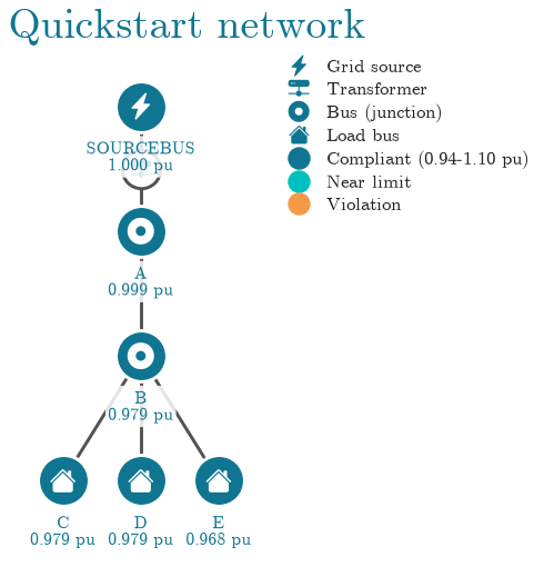
plot_topology() draws the network with each bus coloured by its voltage status.

from popo.plotting import line_style
from popo.plotting.network import plot_topology, topology_from_dss

line_style.configure(latex=False)
plot_topology(topology_from_dss(circuit.dss), title="Quickstart network", figsize=(5.0, 3.6));

findfont: Failed to find font weight bold for cmr10, now using 400.

Simulate a day

To step through time, each load follows a daily profile. Here every house follows the same demand shape, with peaks in the morning and evening, and house E gets a 10 kVA rooftop PV system that follows a clear-sky solar shape. Both profiles have 48 half-hourly values.

import numpy as np

hours = np.arange(48) / 2
demand = 0.25 + 0.35 * np.exp(-(((hours - 8) / 1.5) ** 2)) + 0.75 * np.exp(-(((hours - 19) / 2.0) ** 2))
solar = np.clip(np.sin(np.pi * (hours - 6) / 14), 0, None)


def as_mult(values):
    return ",".join(f"{v:.3f}" for v in values)


circuit.command(f"New Loadshape.Demand npts=48 interval=0.5 mult=({as_mult(demand)})")
circuit.command(f"New Loadshape.Solar npts=48 interval=0.5 mult=({as_mult(solar)})")
for house in ["C", "D", "E"]:
    circuit.command(f"Edit Load.House_{house} daily=Demand")
circuit.command("New PVSystem.PV_E phases=1 bus1=E.3 kV=0.23 kVA=10 Pmpp=10 irradiance=1 daily=Solar");

solve_time_series() solves the 48 steps. It records the transformer at every step and, when you pass buses, the voltage at each of those buses too. The report says whether every step converged.

report = circuit.solve_time_series(48, buses=["c", "d", "e"])
report.converged

True

report.records has one row per step and transformer: active, reactive and apparent power at the secondary winding, the busbar voltage, and the power at the head of the feeder. At midday the PV output exceeds the three houses’ demand, so the transformer’s active power turns negative.

report.records[["step", "trafo", "p_kw", "q_kvar", "s_kva", "v_lv_pu"]].iloc[20:28]

	step	trafo	p_kw	q_kvar	s_kva	v_lv_pu
20	20	lvtr	-1.208	2.298	2.596	1.0
21	21	lvtr	-2.608	2.075	3.333	1.0
22	22	lvtr	-3.460	1.993	3.993	1.0
23	23	lvtr	-3.955	1.989	4.427	1.0
24	24	lvtr	-4.292	1.993	4.732	1.0
25	25	lvtr	-4.473	2.004	4.902	1.0
26	26	lvtr	-4.531	2.008	4.956	1.0
27	27	lvtr	-4.474	2.004	4.902	1.0

voltage_traces() returns each bus’s voltage over the day.

from popo.plotting import tokens

traces = report.voltage_traces()
colors = {"c": tokens.TEXT_MUTED, "d": tokens.HIGHLIGHT, "e": tokens.PRIMARY}

fig, ax = line_style.new_panel()
for bus, trace in traces.items():
    ax.plot(hours, trace, color=colors[bus], lw=line_style.LINE_WIDTH, label=f"House {bus.upper()}")
line_style.hour_axis(ax)
line_style.set_y_axis(ax, *traces.values())
ax.set_ylabel("Voltage (pu)")
line_style.finish(ax)
line_style.legend_below(ax, ncol=3)
line_style.show(fig)

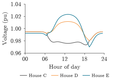
While the PV system generates, the voltage at house E rises to about 1.02 pu. The unbalanced flow also moves the other phases: house D rises and house C falls, so a single-phase installation changes the voltage seen by customers on other phases. event_summary() reports, for each bus, how far and for how long its voltage left the band; here every house stays within it.

limits.event_summary(traces)

	name	v_mean_pu	v_min_pu	v_max_pu	v_std_pu	over_steps	over_severity_pu	over_longest_steps	under_steps	under_severity_pu	under_longest_steps
0	c	0.985	0.973	0.995	0.008	0	0.0	0	0	0.0	0
1	d	0.998	0.980	1.011	0.009	0	0.0	0	0	0.0	0
2	e	0.999	0.970	1.023	0.015	0	0.0	0	0	0.0	0

Next steps

• Key concepts explains per unit, phases, statutory limits and observability.

• The user guide covers each module in more depth.

• The tutorials work through three studies on real feeders, including hosting capacity and state estimation.